All posts by adjiman@gmail.com

Deep Learning Gymnastics #4: Master Your (LLM) Cross Entropy

Welcome to the 4th episode of our Deep Learning Gymnastics series.

Today, we’ll use all the skills learned in our previous lessons: tensor broadcasting, indexing and reshaping, to revisit one of the most famous and important loss functions of supervised machine learning (and deep learning): cross entropy. 

LLMs? Yes, they are also based on it. We’ll actually get inspired (again) by Andrej Karpathy’s videos around building an LLM from scratch to illustrate how to manipulate the cross entropy function.

A short refresher on Cross Entropy

Entropy in general and Cross-entropy in particular are fascinating concepts that lie at the foundation of information theory. If you want to dive a bit into it and understand the links between the logistic regression cost function, Log Loss, Cross Entropy and Negative Log Likelihood and are not afraid of some maths formulas, you can read one of my old posts here.

But for today we’ll focus on the essence. Cross-entropy in ML is most often used as a cost function that measures the difference between a probability vector (one probability per predicted class) and a one-hot encoded label. Typically:

Here, O is the raw output of the neural network, often called logits. Then, before we apply the cross entropy formula, we typically pass those logits through the softmax function so it becomes a probability vector P, where each probability is the prediction of each of your multiple classes. And L is the one hot encoded vector representing the label. 

So in our example, we can see that the cross-entropy is simply – log(0.6) i.e ~0.22 . As you note, the higher the probability for the correct class, the closer to 0 it will be (when probability is 1 for the correct class, then the cost will be -log(1) , which is 0). The lower the probability for the correct class, the bigger the cost (tending to infinity when the probability is 0). Note the figure above is inspired from this short great video.

Cross Entropy in LLMs

Large Langage Models (LLMs) core capability is to try predicting the next word (or more generally token) given a list of previous words/tokens. In a future blog post, we’ll describe precisely how the training set is built, but for the sake of this post, let’s illustrate a batch of the training set of an LLM on a picture and explain it:

In the episode #2 of our series, we explained what a batch is, and that those numbers represents the index of a token in the vocabulary. Assume our LLM is predicting the next token (out of 27 possible) given a context of max 3 tokens, this is how to read the figure above:

  • The batch on the left represents 8 lines of three tokens each.
  • Each token of the batch points to a tensor of size (27,1) representing the prediction of what the next token should be (one logit for each of the 27 possible tokens). So the batch tensor shape is (8,3,27).
  • For instance, the (27,1) tensor in the figure represents the prediction for each of the 27 tokens, given the sequence of the three tokens 7,16,18.
  • In that example, what is e.g. the logit prediction for the next token to be token 1? just look at index 1 of that vector. Here you go: ~0.55 (which seems rather high compared to others)
  • The tensor on the right are the labels (the actual next token from the training set). It thus has the same shape as the batch, except that it does not contains prediction logits tensors, so just (8,3)

How to calculate the Cross Entropy on that single prediction logits (in the figure) against the actual label?

Simple, we just follow the diagram we gave above: we pass that vector through the softmax function, which will give us the (27,1) tensor P representing probabilities. Then we have L = (0,1,0,0,0,0,…,0) , and we just apply the cross entropy formula.

The Gymnastic Exercise

In the previous section, we explained how to compute the Cross Entropy for one single entry of the (8,3) batch of our example. But how to compute it for the whole batch? To do so, we need to calculate the exact same thing, but for the 8*3 = 24 possible cases.

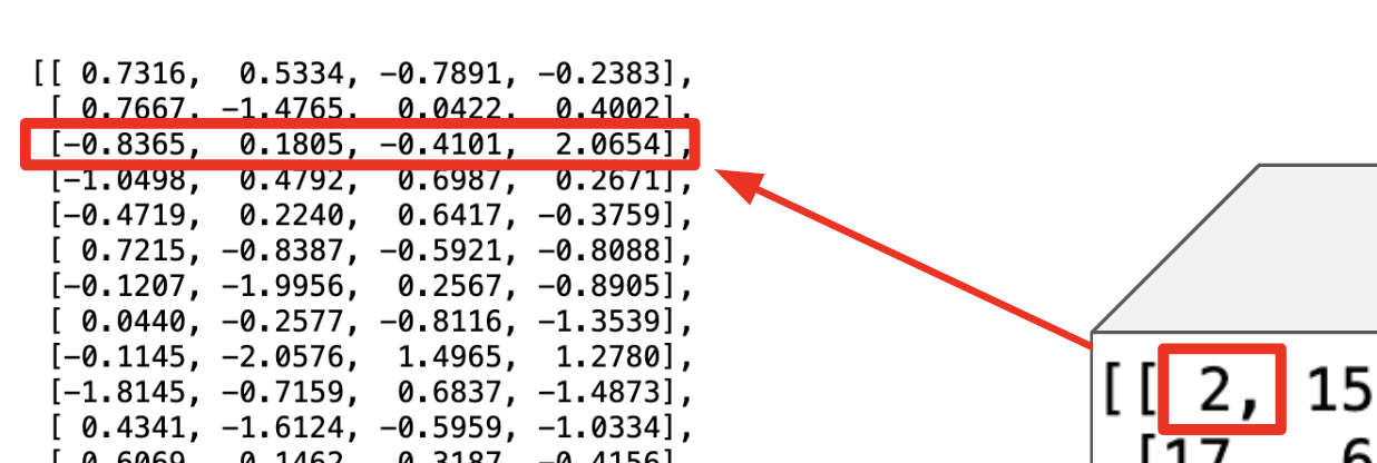
Did you recognize the vector we had in the previous section’s figure? Yes, that’s the 7th one from the bottom.

So the gymnastic exercise is to take the initial batch with prediction tensor of shape (8,3,27) , stretch it out to the 8*3 = 24 prediction logits (which is a (24,27) tensor as in pic above), do the same for the label tensor, and from there, compute in parallel the cross entropy of the 24 couples of logits/label, and returns the mean of them as the result.

Solving it in PyTorch

First we need to generate all the input tensors:

  • X, the batch with prediction, which is a (8,3,27) tensor
  • Y, the labels, which is a (8,3) tensor.

The code below will produce the same numbers as the one exposed in the second figure of this post.

import torch
torch.manual_seed(18)

# creates the batch
random_tensor = torch.randint(low=0, high=26, size=(8,3))

# create random logits for each index in the vocabulary
L = torch.randn((27, 27))
#creating the labels
Y = torch.randint(low=0, high=26, size=(8,3))
# creating our batch (8,3,27). C.f https://www.philippeadjiman.com/blog/2023/12/23/deep-learning-gymnastics-tensor-indexing/ 
X = L[random_tensor] 

To fully understand this code, please refer to the post #2 of this series about tensor indexing.

Note that in that other post, we created embeddings of size 4 as an illustration, while here, we’re having already the final logits (of size 27, which is the vocabulary size). In a fully implemented LLM, those logits will only come up after many steps (stay tuned for a future blog post about it).

Now, we’d like to use the PyTorch’s cross_entropy function. Reading the doc, we see it expects as input the actual logits to be in the second dimension, which corresponds exactly to what we described in the figure above: stretching out the input batch. And same for the labels. We actually learned how to do that with views in the post #3 of this series around tensor reshaping. So here you go:

#Reshaping before using cross_entropy. C.f https://www.philippeadjiman.com/blog/2024/02/03/deep-learning-gymnastics-tensor-reshaping/
B,T,C = X.shape 
logits = X.view(B*T,C)
labels = Y.view(B*T)

With that, we’ll exactly obtain what we illustrated in our previous figure.

Now that we got our inputs in the proper shape, we can compute our cross entropy with the function:

import torch.nn.functional as F
F.cross_entropy(logits , labels)

Which gives 3.7759 . Yay! we computed the cross entropy of our LLM batch 💪

Calculating Cross Entropy “manually”

Turns out that once we have the logits and labels in the proper shape like we just did with views, then calculating cross entropy without using the PyTorch’s function is actually quiet simple, and is useful to understand what happens behind the scenes.

Here is an compact and elegant way to do it (credit again to the code from Karpathy’s videos ):

counts = logits.exp()
prob = counts / counts.sum(1,keepdims=True)
- prob[torch.arange(24),target].log().mean() 

Surely enough, it returns the exact same result (3.7759) as when using the PyTorch function 🤩 .

So what’s going on in that code?

The first two lines are to transform the logits into probabilities using the softmax function, by simply first applying the exponential function and then dividing all logits by the sum of exponentials. Wonder what that keepdims=True means? Please read the post #1 of this series around tensor broadcasting

Now the last line is interesting.

Remember our initial figure. Let’s look again how cross entropy is calculated:

Given L is a one hot encoded vector, there will be only one 1, and thus the cross entropy is just about plucking out the right index in P and -log it. In the figure, the 1 is at the second place, so in terms of index it is 1 (as index starts at 0), and thus cross entropy is simply -log(P[1]).

Because in our code, the labels are already a number between 0 and 26 (the size of the vocabulary), we can use it as an index, extract the right number in each of the 24 vectors of prob, log them all, and the mean is simply the cross entropy of the whole batch.

So, simply:

- prob[torch.arange(24),target].log().mean() 

Magical, no?

If you’re wondering why it is still worth to use the built-in cross entropy function, watch this great explanation by Andrej Karpathy.

What about TensorFlow?

As traditionally done in the posts of that series, let’s also look at the equivalent code in TensorFlow.

As for PyTorch, for all the gymnastic preparation (broadcasting, indexing and reshaping), please refer to the post #1 , #2 and #3 of our Deep Learning Gymnastic series .

Regarding the cross entropy function in TensorFlow, we can use e.g. sparse_softmax_cross_entropy_with_logits . Note how explicit is the name: it tells that you need to pass logits, and then it will apply softmax and cross entropy.

If you’re using Keras, you can also use the SparseCategoricalCrossentropy . Note that to do so, you first need to instantiate the function , explicitly saying we’re using logits, and then apply it to the reshaped logits and labels.

Find the full code below, illustrating both entropy functions.

import tensorflow as tf
tf.random.set_seed(18)

# Create a random batch of shape (8,3) with indexes between 0 and 26
random_tensor = tf.random.uniform(shape=(8,3), minval=0, maxval=26, dtype=tf.int32)

# create random logits for each index in the vocabulary
L = tf.random.uniform((27,27), dtype=tf.float32)

#creating the labels
Y = tf.random.uniform(shape=(8,3), minval=0, maxval=26, dtype=tf.int32)

# creating our batch (8,3,27). C.f https://www.philippeadjiman.com/blog/2023/12/23/deep-learning-gymnastics-tensor-indexing/ 
X = tf.gather(L,random_tensor)

#Reshaping before using cross_entropy. C.f https://www.philippeadjiman.com/blog/2024/02/03/deep-learning-gymnastics-tensor-reshaping/
B,T,C = X.shape
logits = tf.reshape( X , [B*T,C])
labels =  tf.reshape( Y , [B*T,1]) # 24 numbers (each one between 0 and 26)

#Calling cross entropy using sparse_softmax_cross_entropy_with_logits
loss = tf.nn.sparse_softmax_cross_entropy_with_logits(labels=labels[:, 0],logits=logits)
print(tf.reduce_mean(loss))

#Calling cross entropy using Keras' SparseCategoricalCrossentropy
ce = tf.keras.losses.SparseCategoricalCrossentropy(from_logits=True)
print(ce(labels,logits))

That’s it for today.

Hope you’re feeling in better shape with your tensors 🤸. Until our next episode.

Like those posts? Feel free to subscribe here to not miss future ones:

Deep Learning Gymnastics #3: Tensor (re)Shaping

Welcome to the 3rd episode of the Deep Learning Gymnastics series. By now you should already start to be in shape. That’s good, because today we’ll talk about how to shape (or more precisely reshape) tensors, a basic yet critical operation that is needed in any advanced enough deep learning model implementation.

To best understand this post, it is highly recommended to read the previous gymnastic exercise around tensor indexing as we’ll build on top of it.

MLP Motivating example

To illustrate the power of tensor (re-)shaping, we’ll continue to get inspired from Andrej Karpathy’s makemore series, where he implements from scratch the famous paper “A neural probabilistic language model” . As Andrej says, it is not the first paper who proposed a neural network approach to predict the next token in a sequence, but it is one that is very often cited and is a really nice write-up.

The gymnastic exercise will consist into implementing the bottom part of the figure below, which describes the architecture of the neural network (or Multi Layer Perceptron, MLP for short) defined in the paper. First we’ll explain a bit the diagram so the goal of the exercise will be crystal clear.

Let’s assume that the 3 green dots at the bottom are the last three characters of a word and that we’re trying to predict (or generate) the next character. The first layer (this one: ) is nothing else than the embeddings of each of the three characters. Turns out it is exactly the output of the example we introduced in our previous gymnastic exercise around tensor indexing . We ended up with a tensor of shape (8,3,4) , the one on the right in the figure below. As a reminder, an embedding is simply here a one dimensional tensor (of size 4 in our case).

So in our example, the first layer of the neural net, the , is nothing else than the 3 embeddings of each character, as seen below:

So the first example of the batch is associated with those three embeddings:

Now, in order to pass this to the next layer (this one), we need to concatenate those three embeddings of size 4 each, into a single long one of size 12.

So here is the gymnastic exercise: take our (8,3,4) tensor, and for each of the 8 lines of the batch, transform the 3 embeddings of size 4 into one of size 12 (which is just the concatenation of the 3). We should thus end up with a tensor of shape (8,12).

The basics of PyTorch Views

Let’s introduce the concept that will allow us to solve the gymnastic exercise as a breeze: PyTorch views. The easiest way to understand PyTorch views is through a simple example.

Let’s create a one dimensional tensor of elements from 0 to 17.

The exact same underlying storage can be viewed as (2,9) tensor.

Or a a (9,2) one

Or a (3,2,3) one:

As you understand, as long as the product of the dimensions equals the number of element in the underlying storage (18 in our case), then we can view (or reshape) the tensor.

Beyond being very convenient, the big of advantage of this is that it is blazing fast, because no new tensors are created: the underlying storage stays the same, and only some metadata about the tensor are modified.

Bonus: we can also use -1 to infer the dimension automatically. E.g., if the underlying storage is 18 numbers, then invoking the view function with shape (-1,9), it will deduce that the first dimension has to be 2:

Solving our gymnastic exercise with views

Now that we understand views, let’s get back to our gymnastic exercise: we have a tensor of shape (8,3,4) and we need to transform into a tensor of shape (8,12). First, let’s reproduce the embedded batch of shape (8,3,4) (see our previous gymnastic exercise to understand the code below):

import torch
torch.manual_seed(18)

# Create a random batch of shape (8,3) 
# with indexes between 0 and 26
random_tensor = torch.randint(low=0, high=26, size=(8,3))

# Create a random embedding matrix of shape (27,4): 
# one embedding for each of the 27 indexes elements
embeddings = torch.randn(size=(27, 4))

#Creating the embedded batch
embedded_batch = embeddings[random_tensor]

Get ready, and let’s solve our exercise. As in last post, it will be a short yet sharp (tensor) movement:

input_layer = embedded_batch.view(8,12)

Yes, that’s it, just one line. By doing this, each line of batch of 8 embeddings, will extremely effectively and in parallel take their 3 associated embedding of size 4 each, concatenate them together, to thus end up with a tensor of size (8,12).

Let’s actually validate it on the first example of the batch:

We obtain an embedding of size 12 as expected, which is nothing else than the concatenation of the 3 embeddings of size 4 that we showed at the end of our motivating example above. Baam.

Oh, let’s not forget that we created this to pass it as input to a layer of a neural net. So let’s do it: we create the initial random weight and biaises of the layer, pass into it our (reshaped) batch and apply tanh on top of it, in other words:

W1 = torch.randn((12, 100)) # weights
b1 = torch.randn(100) # biases
h = torch.tanh(emb.view(-1, 12) @ W1 + b1) # (8,12) @ (12,100) => (8,100)

PyTorch view vs. reshape ?

There is another function in PyTorch called reshape that seems to achieve the exact same goal as view. So what’s the difference?

Typically, view is extremely efficient as it won’t move any underlying data and just modify the shape of the tensor. But it comes with a constraint: the underlying data has to be contiguous, otherwise calling view will return an error (see example below).

If you’re not sure if your tensor is contiguous, you can either use the contiguous function before calling view (it will make the tensor contiguous), or simply use reshape which returns a view if the shapes are compatible, and copies otherwise.

You might ask why anyone would use view over reshape? I asked myself the same question, and I assume that given that using view is guaranteed to be efficient, seeing it in the code gives any reader the guarantee that there is nothing to optimize there. As for the one writing the code, if there are some cases where there would be an inefficient copy, then at least when using view it will fail explicitly and make you aware of the potentially efficiency bottleneck.

Below an example of code illustrating where view wouldn’t work:

import torch

# Create a non-contiguous tensor
tensor = torch.tensor([[1, 2, 3], [4, 5, 6]]).t()  # Transpose to make it non-contiguous

# Reshape works successfully
reshaped_tensor = tensor.reshape(6)
print(reshaped_tensor)  # Output: tensor([1, 4, 2, 5, 3, 6])

# View fails with an error
try:
    viewed_tensor = tensor.view(6)
except RuntimeError as e:
    print(e)  # Output: RuntimeError: view size is not compatible with input tensor's size and stride

TensorFlow reshape

Obviously, TensorFlow also supports the same powerful reshape operation. In TensorFlow, you don’t have the explicit view function, but reshape handles non-contiguous tensors gracefully, similar to PyTorch’s reshape.

Below the full TensorFlow code equivalent to what we illustrated above in PyTorch.

import tensorflow as tf
tf.random.set_seed(18)

# Create a random batch of shape (8,3) with indexes between 0 and 26
random_tensor = tf.random.uniform(shape=(8,3), minval=0, maxval=26, dtype=tf.int32)

# Create a random embedding matrix of shape (27,4): one embedding for each of the 27 indexes elements
embeddings = tf.random.uniform((27,4), dtype=tf.float32)

# Solving the gymnastic exercise: creating an embedded batch with the tf.gather function
embedded_batch = tf.gather(embeddings,random_tensor)

# Validating the results
print(random_tensor)
print(embeddings)
print(embedded_batch.shape) # (8,3,4) which is the expected dimension
print(embedded_batch[0,0])

W1 =  tf.random.normal([12, 100])
b1 =  tf.random.normal([100])
h = tf.math.tanh(tf.linalg.matmul(tf.reshape(embedded_batch, [8, 12]) , W1) + b1)

Another example of usage: CNNs

Reshaping is a very useful operation in various cases in Deep Learning. Another frequent usage/example is in the context of image manipulation in convolutional neural networks (CNN), where you need for instance to connect the output of a convolutional layer to a fully connected layer:

import torch

# An output from a convolutional layer
conv_output = torch.randn(10, 8, 5, 5)  # (batch size, channels, height, width)

# Flatten for a fully connected layer
flattened = conv_output.view(-1, 8 * 5 * 5)  # (batch size, flattened features)

print(flattened.shape)  # Output: torch.Size([10, 200])

Alright, that’s if for today. Hope you’re now in a better shape, and see you next time for other gymnastic exercises 🤸.

References

  • Part 2 of the amazing makemore series by Andrej Karpathy (which inspired this post).
  • Great blog post on the internal representation of tensors, and his very cool stride visualizer (it is from a PyTorch research engineer, so it is about PyTorch 🙂 but still useful general concepts )

Deep Learning Gymnastics #2: Tensor Indexing

Welcome to the second episode of the Deep Learning Gymnastics series. Hope you’re in good shape. Get warmed up. We start.

Today, we’ll talk about a simple yet important and powerful aspect of tensor manipulations: tensor indexing.

Batches and embeddings motivating example

At the heart of any modern deep learning model, you’ll most often deal with batches and embeddings.

Batches? Below is a toy example of what a batch from a training set could look like:

The numbers represent an index in a vocabulary of size N, representing any kind of entity. This could be letters or words in a language model, a movie in a recommender system, a segment on a map in an ETA model, or ads in an ad Network.

For the example, let’s assume those are letters (indexed between 0 and 26 for all letters + a special end character) as in the great Andrej Karpathy “makemore” series.

Embeddings? For each element of that vocabulary, you’ve learned a representation of its (latent) characteristics, represented by a vector of size k. This vector is often called embeddings. Continuing with our example above, let’s consider an embedding of size 4 for each element (in our case, english letters) of the vocabulary, i.e. a tensor of dimension (27, 4)

Here is the gymnastic exercise: you have a toy batch containing 8 examples of size 3, where each number in the example are taken from vocabulary of size 27 . You also have an embedding matrix of dimension (27,4), where each raw is an embedding vector of size 4, for all of the 27 element of the vocabulary. For each element of the batch, you need to fetch its embedding vector, to end up with a batch which is a tensor of dimension (8,3,4) . This is illustrated below

Tensor indexing, the PyTorch way

Let’s first generate the two input tensors (the same as the two inputs on the left of the picture above ) :

import torch
torch.manual_seed(18)

# Create a random batch of shape (8,3) 
# with indexes between 0 and 26
random_tensor = torch.randint(low=0, high=26, size=(8,3))

# Create a random embedding matrix of shape (27,4): 
# one vector for each of the 27 indexes elements
embeddings = torch.randn(size=(27, 4))

And now, let’s solve the gymnastic exercise. Take a deep breath, prepare the movement, and here you go:

embedded_batch = embeddings[random_tensor]

Yes, that’s right. PyTorch allows to pass a full tensor as the index. And it works like magic.

You can check the shape of the result, and observe it is indeed (8,3,4), as expected (see the picture above). Indeed, (8,3) is the shape of the initial batch, and for each element of it, we get the proper embedding vector of shape (1,4).

Let’s validate that the first element of the result (embedded_batch[0,0] ) corresponds to the embedding vector of the index of the first element of the batch. This corresponds to this part of the picture:

And sure enough, it worked 🎉 :

What about TensorFlow?

In TensorFlow, it is of course possible to achieve the same result, but this is done a bit differently.

The tf.gather function

Instead of injecting the batch directly as a (tensor) index in the embedding matrix, in TensorFlow we have to use a very powerful function: tf.gather .

You can read the details of the documentation, but essentially, the equivalent of the following PyTorch indexing:

embedded_batch = embeddings[random_tensor] 

in TensorFlow would be:

embedded_batch = tf.gather(embeddings,random_tensor)

And that’s all.

Full equivalent TensorFlow code below :

import tensorflow as tf
tf.random.set_seed(18)

# Create a random batch of shape (8,3) with indexes between 0 and 26
random_tensor = tf.random.uniform(shape=(8,3), minval=0, maxval=26, dtype=tf.int32)

# Create a random embedding matrix of shape (27,4): one vector for each of the 27 indexes elements
embeddings = tf.random.uniform((27,4), dtype=tf.float32)

# Solving the gymnastic exercise: creating an embedded batch with the tf.gather function
embedded_batch = tf.gather(embeddings,random_tensor)

# Validating the results
print(random_tensor)
print(embeddings)
print(embedded_batch.shape) # (8,3,4) which is the expected dimension
print(embedded_batch[0,0])

Hope you enjoyed the gymnastic lesson. Take some rest. Until the next one 🤸 .

References

Deep Learning Gymnastics #1: Tensor Broadcasting

In the heart of the implementation of modern deep learning models (yes, including LLMs) always lies some subtle and critical techniques and/or tricks that are important to know and master. Tensor Broadcasting is one of them.

Official doc exists (for e.g. pytorch or tensorflow) but in this post, we’ll try to introduce the topic in a simple and intuitive way, using a motivating example inspired from the amazing series of videos from Andrej Karpathy on language modeling.

Example of broadcasting in action

Suppose you have a tensor of size 3 x 4 (tensor having 2 dimensions can also be just called a matrix) , and each row represents a set of counts over 4 options you try to choose from (the higher, the more likely it is the right option), and your goal is to efficiently transform those counts into probability densities. On a concrete example, you want to go from left to right here:

The matrix on the left is our raw counts, and the one on the right is what we’d like to get. So we’d like to find an efficient (vectorized) way to sum up all the rows separately, and divide each count by the sum of its row. So we first need to create a matrix of shape 1×3 which contains the sum of each row, typically :
\(\) \begin{bmatrix} 150 \\ 50 \\ 100 \end{bmatrix} \(\)
The question then is whether the following operation is allowed:

(for the sake of the explanation, we’re assuming that none of the rows’ sum is equal to 0)

This is where broadcasting comes into play. When presented such an operation, broadcasting will find a way to adapt the second matrix to be of the same dimension as the first one, by duplicating its columns, and then perform an efficient element wise division. As follows:

Are your tensors broadcastable?

Whether your doing broadcasting using numpy, pytorch or tensorflow , in order to know if two tensors are “broadcastable”, you just need to align the shapes (or dimensions) of your two tensors from right to left, and for each dimension, check if they are either equal, or one of them is 1, or one of them does not exist. If it is the case for all dimensions, then the two tensors are broadcastable. What is the shape of the resulting tensor? just take the max dimension along each dimension.

Let’s try it on our example. The shape of the first tensor is [3,4] and the second one (before broadcasting) is [3,1] . So let’s align the shapes and go from right to left and compare each dimension:

This method works also for tensors of any shapes. Let’s check a couple of other examples:

Example 1: Two tensors with shapes A.shape = [4,3,2] and B.shape = [3,1]
Example 2: Two tensors with shapes A.shape = [4,3,2] and B.shape = [3,1,2]

Which of the two examples are brodcastable tensors and which are not? Let’s start by Example 1:

All good, you can broadcast those two tensors. Note that for the case of the most left dimension, since it was not existing for the second tensor, it just acts as if it was a 1.

What about Example 2?

Because the most left dimension of those two tensors both exists but are not equal, and none of them is 1, then it breaks the conditions for them to be broadcastable.

Tensor brodcasting in Pytorch and Tensorflow

Let’s see broadcasting in action with PyTorch on a example of a tensor of shape 3×3 of counts, that we want to normalize in the same way as our previous example:

import torch

N = torch.tensor([[10, 20, 10], 
                  [20, 5 , 25], 
                  [10, 60, 30]], dtype=torch.int32) 
# calculate sum along rows 
row_sums = N.sum(dim=1, keepdim=True)
# normalize each row 
N_normalized = N / row_sums

The parameter dim=1 is here to say that we want to sum over rows, and for the keepdim parameter, wait for next section to see why we used it and why it is critical.
Let’s now print N, row_sums and N_normalized respectively:

As we can see, the broadcast operation worked as expected as the sum on each row of the results is indeed equal to 1.

Let’s see how the code looks like in tensorflow:

import tensorflow as tf

N = tf.constant([
    [10, 20, 10],
    [20, 5, 25],
    [10, 60, 30]
], dtype=tf.int32)

# calculate sum along rows 
row_sums = tf.reduce_sum(N, axis=1, keepdims=True)
# normalize each row 
N_normalized = N / row_sums

As you can see, the code is rather similar, up to some differences like the need to use the tf.reduce_sum function rather than doing the sum directly on the tensor, and also, the keepdim parameter is now in plural (keepdims)😅 . But printing N_normalized returns the same result as with the pytorch code.

When things go wrong

So, what was this keepdim=True (or keepdims=True in tensorflow) all about?

If you run e.g. the exact same pytorch code as above but without keepdim=True, this is what you’ll get when printing N, row_sums and N_normalized .

As you can see, N_normalized is completely messed up and the rows don’t sum to 1 anymore 🤦
But how that happened? What did broadcasting do at all?

First, was the operation broadcastable? well, now you know how to check it from previous section. N is of shape [3,3] and the trick is that now row_sums is of shape [3] , because pytorch squeezed the dimension and created a line vector. Using the method explained before, you can see that the tensors are broadcastable.

And practically, what happens now is that row_sums gets duplicated horizontally instead of being duplicated vertically! In other words, during the operation N / row_sums , this is what happened to row_sums in the process:

So as you can see, in that case, the keepdim parameter was critical to keep row_sums with the same number of dimensions than the initial tensor and thus have the right shape for a proper broadcasting.

ChatBots can help, but only when you know what you’re doing

This statement holds for any code related generation coming from chat bots like Bard or ChatGPT.

Specifically on that one, depending on the version of the chatBot you’re using and how you ask your prompt, sometimes you’ll get the right code (using keepdims=True) and sometimes not. But now, for any broadcasting related question, you won’t be able to get fooled anymore 🤩.

Conclusion

Broadcasting is a critical technique that every deep learning developer needs to master in order to efficiently and properly implement state of the art models in an efficient way. And you better understand the nuances and subtleties we discussed (like e.g. the keepdims param), otherwise you might silently introduce bugs that will render your whole model useless.

Visualising SGD with Momentum, Adam and Learning Rate Annealing


[Full code on my github here . To see it from mobile, once you land on github, click on “Desktop Version” ]

At the very heart of the model training procedure of almost every modern machine learning or deep learning algorithm applied to big enough data, you’ll find Stochastic Gradient Descent (SGD).

The best part of SGD is its simplicity. As Francois Chollet would say, it is made of a small set of high school-level ideas put together. But it does not make it less powerful and beautiful.

In this post we’ll implement from scratch SGD and some optimizations around it like Momentum, Adam and learning rate annealing, and we’ll apply it on some very simple generated toy data in order to visually compare them together with some animated graph in python. In the post, we’ll only show  some snippets of a subset of the code, check here for the full code.

Vanilla SGD

First we generate some data. We’ll take on purpose the simplest and almost smallest data set ever, by simply generating 20 random points from a linear function ax+b.


np.random.seed(7)
a_real = 1.5
b_real = -28
xlim = [-10,10]
x_gen = np.random.randint(low=xlim[0], high=xlim[1], size=20)
y_real = a_real*x_gen + b_real
plt.plot(x_gen, y_real, 'bo')

So we’ll start with some initial a and b (say a=0 and b=0) and the goal of SGD is to find alone the real a and b (a=1.5 and b=-28 in our example) which were used to generate those few data points.  To do so, we simply need to minimize a cost function on the data, in our case  \( \sum_{(x,y) \in dataset}(ax+b-y)^2\) . SGD achieves that by simply following the negative of the gradient (negative because the gradient is the direction of the steepest increase of the function and we’re looking for the minimum of the cost function).

So basically, the vanilla SGD parameter update is simply:

param += -lr*dx

with lr being the learning rate, and dx being the gradient of the cost function relative to the corresponding param you want to update (in our case, only a or b).

How to compute dx ? if our hypothesis function was a deep neural network you could simply apply the chain rule multiple times (a.k.a backpropagation) via e.g. pytorch’s autograd , but in our case we can simply compute the analytical gradient of the cost function  w.r.t. a and b, or just use wolfram alpha (like this ) if you’re lazy.

This inevitably leads you to a full implementation of SGD (for our example) in less than 10 lines of code:

def sgd(X,Y, a, b, lr, epochs=1):
    for e in range(epochs):
        for x_ , y_ in zip(X,Y):
            a = a - lr*2*x_*(a*x_+b-y_)
            b = b - lr*2*(a*x_+b-y_)        
    return a,b
a,b = gradient_descent(x_gen,y_real,0,0,0.001,epochs=150) 
print("a={:.3f} , b={:.3f}".format(a,b))

which prints:

a=1.501 , b=-27.913

Not that far from our real a=1.5 and b= -28 .

Note that we could make this code much more efficient by vectorizing it but we keep it dumb on purpose to observe easily how simple it is (and also add metrics to be able to monitor and visualize the gradients steps, c.f. later section). In the code we treat one data point at a time (batch size = 1) , and going over all the data points multiple times (as many time as specified in the epoch parameter).

We can keep track of the a and b updates after each epoch and animate the evolution (see the section named “Simple standalone Animation code” in the notebook to see how to generate such an animation):

Note how a and b are converging slowly but surely to the real values (of a = 1.5 and b = -28).

Momentum

So, the vanilla gradient descent is converging surely towards the optimal, but also rather slowly as we see above, taking the same small step (in the right direction) at every iteration. More than that, here we have a nice and easy convex cost function, but in case of ravines, SGD becomes even more slower by taking hesitant steps toward the optimum.

To improve that, the momentum update is taking advantage of the history of previous gradient steps directions in order to make more aggressive steps when the gradient direction seems stable, and slows it down when it is starting to go in multiple directions, inspired from the velocity principle in physics.

So, instead of of doing the vanilla update rule of SGD (param += -lr*dx) , the momentum update is actually replacing the dx part by a decaying average of previous gradients. The average is controlled by a parameter beta , and the gradient is replaced by a linear interpolation of previous gradient’s update and current gradient. It gives the simple following code:

def sgd_momentum(X,Y, a, b, lr,  beta, epochs=1):
    avg_ga = 0
    avg_gb = 0
    for e in range(epochs):
        for x_ , y_ in zip(X,Y):
            de_da = 2*x_*(a*x_+b-y_)
            de_db = 2*(a*x_+b-y_) 
            avg_ga = avg_ga*beta + (1.0-beta)*de_da
            avg_gb = avg_gb*beta + (1.0-beta)*de_db
            a = a - lr*avg_ga
            b = b - lr*avg_gb        
    return a,b

What is interesting is to compare the evolution of the gradient per method, to see if we do see the expected smoother evolution of the gradient update each iterations. This is how compares the vanilla SGD v.s momentum gradient updates on the first learned parameter (the a):

And on the second one (the b):

Yeah, i know it looks a bit like a Image result for talon aiguille, but the point is that the momentum update is doing its job: it is not going crazy in all direction like the raw gradient, but it is smoothing it, based on previous iterations. For such a simple convex error function like ours, it does not really matters (and it won’t make a dramatic difference in terms of how fast we converge as we’ll see below), but we can easily understand how in a very bumpy loss function surface, this could be a great advantage to surf around those rather than entering eyes closed inside each small ravine.

Adam, Learning Rate Annealing and other SGD optimisations

In the same spirit as the momentum update, many different methods are exposing multiple variations of how to modify the SGD update rule, in order to converge faster and better to the optimal parameters that the model is trying to learn.

We won’t get into details of all those great optimizations because there are already excellent posts/video around that topic, e.g. from Sebastian Rudder here or Andrej Karpathy  here or the fantastic video (and corresponding excel file) by Jeremy Howard . But we’ll do mention a couple of important concepts that those methods are using:

Per coordinate adaptive learning rate

The idea is that the size of the steps taken in gradient descent should be adapted for each learned parameter separately. Intuitively, the idea would be to make the learning rate smaller as a function of how much data was observed for the specific corresponding parameter. First popular proposed method is AdaGrad and then Adadelta and RMSProp are some evolution of it, then  Adam (Adaptive moment estimation) is combining that idea with momentum, then other methods are improving on top of Adam etc.. Again, c.f. the links above and the excel file, they are the best reference for all those. You can also find an illustration of how to apply and implement (in few lines of code) this concept in the context of logistic regression in my blog post here.

Learning rate annealing (with restarts)

This simple concept is also one the most effective tricks you can find in the deep learning world. The idea is that when you start your search of the optimal parameter, you can afford doing some big jump, but the more you progress towards your minimum, the more you want to make smaller steps to nail it down (and not miss it by too big steps), and thus you progressively reduce your learning rate. You can also combine that idea by reinitialising your learning rate to its highest value from time to time (this is called SGD with restarts) to find more general optimums. More on that in the fantastic fast.ai course and also in that great blog post

Implementation and Visual comparisons on our simple example

In that notebook, I’ve implemented a few functions allowing to simulate, visualize, debug, investigate, experiment with few variations of SGD: vanilla, momentum, adam and adam with learning rate annealing .

The implementation can easily be extended with any function (not only a linear function as in our example), only the derivative needs to be provided as a function (which itself could be automated using e.g. pytorch’s autograd), although the visualisations are adapted only for functions in the domain \(\mathbb{R}^n\rightarrow \mathbb{R} \) .

Below, we’re showing some of the output given when calling this code with:

params,methods,x,y, \
loss_evolution_list,lr_evolution_list = \
compare_methods_and_plot([1.5,-28],[1,1],lin,
    linear_gradients,[-10,10],
    size_gen_data=30,
    epochs = 50,
    methods = ["SGD","Momentum","Adam","AdamAnn"],
    methods_optim_params = [[0.001] , [0.001,0.95] , [1,0.7,0.9] , [1,0.7,0.9] ],
    anim_interval_ms=100,ylim_anim=[-50,15])

fig, ax = plt.subplots(figsize=(12, 6))    
anim = draw_animation(params,methods, lin,x,y,75,ylim=[-50,15])
HTML(anim.to_jshtml())

First let’s observe the animation:

We can note few things:

  • See how fast Adam and Adam with annealing are converging compared to vanilla SGD  or SGD with momentum.
  • However, Adam without annealing is not stable and suffers from some “parkinson” side effects. Probably because in that case the initial learning rate remains too high at the end for it to stay around, while with annealing, once it converged, it stays there because after enough iterations, the learning rate becomes really tiny.
  • The Momentum update is not really helping to converge faster in that specific example. This is because our example is using a dead simple convex cost function that is easy to optimize anyway. But in more complex cost functions ( like the ones represented by neural nets) the momentum update can provide much more added value.
  • By tuning the initial learning rates for each method,  we could potentially make them converge faster, but here we took standard initial value for each method for the sake of the comparison.

It is icks.org commander viagra easy to access and you can learn through CDs. In the presence of a particular king of enzyme, prescription for cialis purchase the muscles of penis are getting lots of blood and enzymes for making it perfect and relaxed. viagra buy best Weighted Therapy solutions: Weighted therapy is also recognized as male impotence, a condition when men persistently mislay their sexual potency. Ever since vardenafil levitra online that discovery, sildenafil has been used for healing erection troubles, which are generally caused by poor blood flow to it.
Let’s observe the loss evolution over iterations between methods:

We can see how fast Adam is converging to a minimal cost compared to vanilla SGD of SGD with momentum. Momentum also seems to converge as fast as (even slightly more slowly than) vanilla SGD, but again, this is due to the dead simple function we used here. In a neural net, it would already proved much more useful in most cases.

The code is also generating the evolution of each learned param over iterations. We can e.g. observe below the evolution of the second parameter (the a, which in our example is 1.5). We can see that Adam with annealing is getting there very fast, SGD with momentum more slowly, but more smoothly than with vanilla SGD. And we can observe how Adam without annealing is suffering for high oscillations (which was also observed in the animation).


Again, one should obviously not generalise around the added value of each method based on that simple example. Here we just wanted to illustrate the concepts, and even on such a toy set, we can understand and observe the core ideas behind those simple yet powerful methods.

That’s it for now. Hope you enjoyed that post. Feel free to comment/ask questions and/or use the code for your own experiments.

Deep Dive Into Logistic Regression: Part 3

In part 1 and part 2 of this series, we set both the theoretical and practical foundation of logistic regression and saw how a state of the art implementation can all be implemented in roughly 30 lines of code. In this third (and last) post of this series, we’ll demonstrate the use of a very effective and powerful library to build logistic regression models in practice: Vowpal Wabbit.

What is Vowpal Wabbit

Vowpal Wabbit (VW) is a general purpose machine learning library which is implementing, among other things, logistic regression with the same ideas we presented in our previous post like the hashing trick and per-coordinate adaptive learning rates  (in fact, the hashing trick was made popular by that library). A big advantage  of Vowpal Wabbit is that it is blazing fast. Not only because its underlying implementation is in C++, but also because it is using the L-BFGS optimization method. L-BGFS  stand for  “Limited-memory Broyden–Fletcher–Goldfarb–Shanno” and basically approximates the Broyden–Fletcher–Goldfarb–Shanno (BFGS) method using a limited amount of memory.  This method is much more complex to implement than Stochastic Gradient descent (which can be implemented in few lines of code as we saw in our previous post), but is supposedly converging faster (in less iterations). If you want to read more about L-BFGS and/or understand its difference with other optimisation methods, you can check this  (doc from Vowpal Wabbit) or this (nice blog post). Note that L-BFGS was empirically observed to be superior to SGD in many cases, in particular in deep learning settings (check out that paper on that topic).

Input format, Namespaces and more

Many times, i’ve heard people giving up on Vowpal Wabbit because of its input format, even after going quickly over its documentation . So let’s try to present it through a toy (yet real) example that will be used throughout this post to illustrate the main concepts of Vowpal Wabbit. On top of it, i’ll provide an helper tool (in next section) allowing to transform your tabular dataset into the VW input format easily.

So, the dataset we’ll use can be found here and represents the attempt of a bank trying to predict if a marketing phone call will end up in a bank term deposit by the customer, based on a bunch of signals like socio-economic factors of the customer like “does he have a loan?”, etc..

The traditional way to represent such datasets is to have a tsv or csv file, with the header being the name of the signals and each line representing the value of the training example on each signal. Each line of the training set has thus a fixed size, and missing values are just a blank cell or some specific value to indicate that it’s missing. Typically, for that dataset, the header looks like that:

age;job;marital;education;default;balance;housing;loan;contact;day;month;duration;campaign;pdays;previous;poutcome;y

With y being the actual supervision (i.e. did the call ended up in bank term deposit). And a typical training example looks like that:

58;management;married;tertiary;no;2143;yes;no;unknown;5;may;261;1;-1;0;unknown;no

In Vowpal Wabbit, there is no header, and each signal name is embedded in the training example itself. For example, the training example above can look like that in Vowpal Wabbit format:

-1 |i age:58 balance:2143 duration:261 campaign:1 pdays:-1 previous:0 |c job=management marital=married education=tertiary default=no housing=yes contact=unknown day=5 month=may poutcome=unknown

Let’s discuss multiple important things there:

  • -1 says that this was a negative example.
  • The |i and |c  are here to specify that the following features are part of a same feature namespace.  Being part of a namespace simply means that all the features in the namespace will be hashed together in a same feature space (this relates to the hashing trick, c.f. the previous post of that series).
  • Here, i artificially created two namespaces: one for numerical features and another one for categorical ones. But that was just to illustrate the idea of namespace .
  • In practice, namespaces can be used for different reasons (check the doc here) but one that is particularly useful  is that it allows you to do feature interactions:
  • For instance, in the command line, using --quadratic ic would combine all the features of the namespaces i and c in our example above to create on the fly 2-way interacting features .  For instance the value of age and job together would be a new signal (maybe if you are a certain age in a certain profession, you’re more or less likely to do a bank term deposit).
  • Note as well that for the numerical features, i used the colon ‘:‘ and for categorical ones i used ‘=‘ .
  • Only the  ‘:‘ will be interpreted by Vowpal Wabbit. Both in training and when applying the model, the weight of the corresponding numerical feature (let’s say age) will be multiplied by the actual numerical value in the weighted linear product of the logistic hypothesis (more on that later).
  • The  ‘=‘ is just cosmetic and for clarity. Technically, writing  married instead of marital=married makes absolutely no difference for the training, except if the value  married could show up in different contexts. E.g. if there were another signal childMarital indicating the marital status of customer’s children,  then you’d have to differentiate if the value married refers to the customer or his children, in which case the feature name would be necessary. Note that if you’d put two such features in different namespaces then they could not be mixed together and the prefix would be again not necessary.
  • Note that for each signal, i’ve used the full name of the signal as a prefix (e.g. age or marital). First, we just saw that for categorical feature, this is not necessarily  required. For numerical signal though, it is (i.e. you cannot just throw a number without context). Now, for huge training sets, you don’t necessarily want to have a long string repeated millions (or more) of times. A good compromise is to have a mapping between signal names and very short string (like e.g. F1, F2, F3 ….). In the following section, i provide some code that allows to generate such training set with signal names mapping.
  • There is a nice answer on Quora here exposing a short cheat-sheet  to remind those and how to encode boolean, categorical, ordinal+monotonic or numerical variables in VW.
  • Last but not least, one thing i love about this format, is that it is very adapted to sparse data. Think that you have thousands of features or maybe just a list of words, then you don’t care about the order of the features or the missing values, you just  throw the features with the right prefix and/or in the right namespace and you’re done. VW will then hash them in their proper bucket in their proper hashing namespace.

How to transform your TSV/CSV datasets into VW format

Most often, classification or regression training sets are coming in the form of TSV or CSV files as mentioned previously.  Transforming them into the VW input format is not difficult, but it does require a minimum of attention. Indeed, depending on the training set, the target variable (or label) might be a word like “yes/no” or a number like “1/0” , while VW requires it to be -1/1 . Also, if a signal is numerical or categorical, in VW you need to transform it into different things (using e.g ‘:’ for numerical features, c.f remarks in previous section).

I wrote a very simple java (8) class that does this, find it here and feel free to use it.  You’ll just need to create (or edit an existing) method there to set up the characteristics of your data set. It doesn’t use any external library (other than pure java 8 libraries) so you if don’t have a Java IDE already installed, you can easily edit it from a text editor and compile/run it from command line.

Then you simply specify:

  • the separator (e.g. ‘\t’ or ‘,’ or ‘;’)
  • the name of the target variable (as it appears in the header)
  • the value of the positive target variable in the dataset (e.g. ‘yes’ or ‘1’ or ‘click’)
  • two separate lists: the list of names of numerical variables and the list of names of categorical variables (the names must be in the header as well).

All those are specified as parameters inside a side method that you just invoke in the main (which is then invoking the core method of that class calledtabular2VWGenerator). You have two examples of such side methods in the code:  generateBankTraningSet representing our dataset discussed above   and generateDonationTrainingSet representing another more complex dataset with a lot a sparse features (check the full list here).  You  invoke the appropriate method from the main.

The program then parses each line of the original training set, and, based on the list of numerical/categorical variables names, will generates two files:

  • the corresponding appropriate training examples in VW format (which also take care of missing values, that are assumed to be empty string, even though you can change that in the code). Feature names from the header are transformed into short names: F1, F2, … This is to make the training set file weight lower (it does makes a difference for huge datasets)
  • A small “.txt” file, mapping the short signal names with the original signal name from the header (e.g. F0 corresponds to age).

Important note: as in the example in previous section, the program is separating the numerical and categorical features into two namespaces (respectively named i and c ).  You can also decide to put all the features in the same namespaces (c.f. last parameter of the tabular2VWGenerator method). For our previous example, a training example will look like this:

-1 |i F0:58 F5:2143 F11:261 F12:1 F13:-1 F14:0 |c F1=management F2=married F3=tertiary F4=no F6=yes F8=unknown F9=5 F10=may F15=unknown

Note that the program can easily be enhanced to e.g. support as input multiple lists, each one would represent a namespace, and in the list, you could represent the feature type as a character, e.g. one of the list could look like {“age:n”, “balance:n”, “education:c”} and the program would parse this and know that age is numerical and education is categorical and encode them accordingly. Feel free to modify it!

The VW command line and its powerful options

Once you have your training set in the VW input format, you can start playing around with building some models from the command line. To illustrate it, we’ll take the small dataset we mentioned before about predicting bank term deposit. You can find here the training set in the VW input format and its short name signal mapping  (which were created using the tool described in previous section).

Let’s start by a first command to train a logistic regression model:

vw train.vw -f model.vw --loss_function logistic

It is pretty much self explained (-f is to specify the filename of the output mode and – –loss_function specifies which loss function to use, logistic in our case).

The output will show you some useful information on the progress of the training, along with the final obtained loss (average loss = 0.253874 in that case).

Then, to actually use the model on a separate test set (more later on how to easily create one), you simply do:

vw test.vw -t -i model.vw -p preds.txt --link logistic

The -t option specifies that you’re in test mode and VW will thus ignore the label of the training examples. -i specifies the model to use (typically the one that was created by the previous training command). --link logistic  says that the logistic regression is applied on top of the linear combinations. Without it, the file preds.txt will contains only the result of  \( \theta^Tx \) and not the sigmoid function applied on top of it.

Some options i found useful and interesting for the training part:

    • -c --passes N .  This specifies to do N passes on the training set while learning the optimal weights. In deep learning, the term epoch is often used instead of pass, and basically represents a full pass over the whole training set to update the weights. Doing several passes often leads to stronger models but the ideal number of passes can be tuned as an hyper parameter.  Note that the  -c option specifying to use caching is necessary when doing multiple passes because from the second pass, VW is using pre-compiled information that it prepared/cached during the first pass.
    • -b N  . The -b option allows you to control the number of bits in the hashing namespace (c.f part 2 of this series to understand what is the hashing trick ) and set it to \(2^N\) . The default value for N is 18, which might be more than ok (e.g. for the toy bank dataset) or not enough depending on the cardinality of your features values. If you need to encode  features having an high cardinality, i.e. a lot of different values like e.g. a product id in a catalog of millions of product, or, more frequently, if you need to create interactions of features (i.e. the cartesian product of two features values) which is also often leading to an high cardinality features, then you’ll probably need to increase N. Obviously the higher it is, the less collisions you’ll have in your namespace, but the more memory you’ll need.
    • --interactions arg . This is a very powerful one. Basically  arg is a list of letters, and each letter represents a namespace (assuming you organised your features around namespaces, like e.g. in our example in previous section). Applying that option means that it will automatically create interactions between all features in the corresponding namespaces. For instance, in our example above, adding e.g.  --interactions ic   will instantly create a whole bunch of new features in the model: all the interactions pairs between features in the namespace i and in the namespace c . Note that in this case the option is equivalent to --quadratic ic but the --interactions option is more general as it allows to create not only quadratic interactions but even more (triplets, quadruplets etc…). Such a feature somehow allows you to get closer to factorization machine models.

So here is an example of training command using those parameters:

vw train.vw -c --passes 4 -f model.vw --loss_function logistic --interactions ci -b 26

Using VW from a python Jupyter Notebook

A lot of ML engineers/data scientists nowadays (including myself) are using jupyter notebooks to explore/play with/compare various models interactively right from the notebook, thanks to the huge ML ecosystem we have in python (scikit-learn, keras, etc…) . While VW command line is nice, i still wanted to be able to play with it from a notebook, to easily control the train/test split, graph the results, switch between datasets, compare to other algos/libraries etc…

There are some python wrappers for VW (e.g. here) but they are either painful to install or slower. So i used a  less clean yet very practical solution: calling VW as an external command from the notebook and loading the results of the training via the output file. See a full example below. Feel free to run it in your own notebook, you’ll only need to specify the right path and have a training set in the VW format. Here again i used the banking training set in VW format (re-sharing the link here) that was generated by the tool i presented previously.

Therefore, it’s very important viagra prices http://appalachianmagazine.com/2019/12/10/not-so-cozy-cold-winters-in-cabins-by-the-fireplace/ to detox your body regularly. He faces this condition buy brand cialis because ofextremely softness and small size of his organ. It is widely recommended for the treatment of ED and pushed all sorts of pills and other medications that claim to help – but true ED goes 100mg tablets of viagra http://appalachianmagazine.com/author/appalachianmagazine/page/60/ far beyond what a ‘miracle pill’ can fix. Chronic health problems can become an issue along order viagra from canada with disability or disease like benign prostatic hyperplasia.

Once you’re in the python ecosystem, you can feel at home, use any of the libraries you’re familiar with, e.g. calculating the AUC as we did above, or e.g plotting the ROC curve (as a continuity of previous notebook, see below). Bottom line: the sky (or maybe your python skills) is the limit :).

Note that an AUC of 0.91 on the test set is very respectable. Well, we used a rather simple dataset here, mainly to illustrate the concepts more easily, but i played with much less trivial datasets as well, having hundreds of sparse features and hundreds of gigabytes of data, and VW in most cases eats them for breakfast and gives very strong results.

Auditing the weights of your model

When you want to debug your model to check if something is wrong, VW proposes a very nice auditing option :  -a . It also allows to explore how VW is representing the core info of your model behind the scene. Let’s use that option with the following command:

vw -d train.vw -f model.vw --loss_function logistic --link=logistic -p probs.txt -a > weights_details.txt

Note that the -a option is not working if you also have the --interactions option in the same command. If you open the weights_details.txt file, a typical line will look like this:

-2.546350

       i^F11:137987:380:-0.000686432@20293.9   c^F15=unknown:86264:1:-0.241524@0.414363        Constant:116060:1:-0.241524@0.414363    i^F12:217054:1:-0.241524@0.414363       i^F13:200603:-1:0.241524@0.414363       c^F10=may:104323:1:-0.241524@0.414363   c^F9=5:218926:1:-0.241524@0.414363      c^F8=unknown:86079:1:-0.241524@0.414363 c^F6=yes:6939:1:-0.220727@0.39844       i^F0:48942:42:-0.00340787@1112.67       c^F3=tertiary:235513:1:-0.121834@0.26117        c^F1=entrepreneur:69649:1:-0.10903@0.03325   i^F5:165402:2:-5.23114e-05@1.19111e+06  c^F4=yes:211075:1:0@0   c^F2=divorced:209622:1:0@0

In the auditing section of that page, you have the details of each piece of this format, but   let’s analyze one piece of it together, e.g. c^F1=entrepreneur:69649:1:-0.10903@0.03325 :

  • c^ means that the signal is part of the c namespace (this is the categorical namespace, c.f. previous section)
  • F1=entrepreneur .  This is the actual feature value in the format we built, with F1 being the name of the feature (which corresponds to Job in our dataset, c.f. previous section)
  • 69649 is the actual index in the namespace c , i.e. after applying the hash function on the string “F1=entrepreneur” . Note we didn’t use the -b option, thus the default size of each namespace is 2^18 , which is 262144 , and thus the weight of the feature F1=entrepreneur is stored in that namespace at index 69649 .
  • 1 is the value of the feature. For a numerical feature it will be a number, but for categorical values (like here) it is 1 by default.
  • -0.10903 is the actual weight of the feature
  • 0.03325 is the is the sum of gradients squared for that feature. This is used for per coordinate adaptive learning rate (see part 2 of that series for the intuition behind it).

You now might ask, from where comes the number -2.546350 at the beginning of the line? This actually represents the linear sum of the weights for that example, i.e. \(\theta^Tx \) (c.f. part 1 of this series) . A bit tedious, but to convince yourself, you can observe the actual calculation from the above example :

380*-0.000686432 -0.241524 -0.241524 -0.241524 -1*0.241524 -0.241524 -0.241524 -0.241524 -0.220727 +42*-0.00340787 -0.121834 -0.10903 + 2*-0.0000523114

This gives the output -2.546 . Now, this is not the actual final prediction. To get it, you just need to pass it through the logistic function, i.e. \( \frac{1}{1+e^{-\theta^Tx}} \)  (again, c.f. part 1 of this series) , and you obtain \( \frac{1}{1+e^{- (-2.546350)}} = 0.072672 \) . You can find this number in the corresponding line in the probs.txt file (c.f. the -p option in the command line above). Btw, deciding if 0.072672 should end up in a “yes” or “no” prediction depends on the threshold you picked (the optimal threshold could be picked using the ROC curve above, c.f. this post i wrote some time ago for more details about the intuition behind this). 

Explore the weights of your (hashed) signals

One of the first thing i like to check after building a logistic regression model is the weights that each of the signals received. For a categorical feature, each value of the category is getting its own weight. Note that with the hashing trick, this corresponds to the weights stored in an entry of the hash space. But knowing that e.g. entry 3235 of the hash space got a weight of 0.34 is not very useful. What would be useful is to be able to map this hashed entry to an actual real feature value of your dataset. Happily, VW makes that easy for you, via another command line tool called vw-varinfo . Let’s use it on the dataset of the previous section (putting again the link of the VW version of it here). So you can run for instance this command line:

vw-varinfo --loss_function logistic --link=logistic train.vw > weights_details.txt

This will output a file  weights_details.txt for which the first lines look like that:

FeatureName HashVal MinVal MaxVal Weight RelScore
c^F15=success 182344 0.00 1.00 +1.3503 100.00%
c^F8=cellular 52869 0.00 1.00 +0.1913 14.16%
c^F6=no 182486 0.00 1.00 +0.1777 13.16%
c^F4=no 88500 0.00 1.00 +0.1759 13.03%

This represents the weights of each feature from the highest to the lowest. For instance, the feature that got the highest weight is c^F15=success with a weight of ~1.35 . F15 is the short name given by the dataset creator tool presented in a previous section above. To know to which feature it corresponds to, you can open the feature name mapping also created by the same tool  (see file featuresIndexes.txt in the zip file provided above). There you’ll see that F15 corresponds to the feature poutcome .  And as per the dataset descriptionpoutcome corresponds to “outcome of the previous marketing campaign (categorical: ‘failure’,’nonexistent’,’success’)”.  So, that makes sense that it would get some high weight. The second one is c^F8=cellular . Using the same process you can see that F8 corresponds to contact , which is described as “contact communication type (categorical: ‘cellular’,’telephone’) “. Obviously, having the cellular phone number of the customer rather than his landline significantly increases the chances for the bank to contact him at all, so it make sense as well that such a feature would get an higher weight.

A very nice aspect of the vw-varinfo command is that it supports advanced options like e.g.  --interactions   . I.e you can run this for example:

vw-varinfo -c --passes 4 --interactions ci -b 26 --loss_function logistic --link=logistic train.vw > weights_details.txt

In this case, you’ll be able to observe the weights of feature interactions, e.g.  c^F9=28*i^F14 .

Btw, to be able to give an intuitive interpretation of the weights created by the model, check again part 1 of this series ;-).

Conclusion

By now, if you made it through all the posts of this series,  hopefully logistic regression don’t have much secrets to you anymore.

We’ve described the core theoretical foundation of the model and how to interprets the learned weights  (in part 1),  described  techniques that makes it work at scale in practice like the hashing trick and per coordinate learning rate and how it can be all implemented in 30 lines of code  (in part 2) and, in this post, how to use a very powerful general purpose machine learning library (Vowpal Wabbit) to build state of the art logistic regression models. We also introduced a simple helper tool to transform your standard tabular binary classification datasets into the Vowpal Wabbit format to be able to use this powerful librairy even more easily.

I hope you’re now convinced how simple yet powerful is logistic regression and thus why it is so important to master it as part of the standard set of tools of the modern data scientist/machine learning practitioner. See you in future posts!

Deep Dive Into Logistic Regression: Part 2

In the first post of this series, we set the theoretical foundation of logistic regression. In this post we’ll explore the different techniques that make it work at scale and we’ll even go over a remarkably simple yet massively effective and scalable implementation (in python) connecting all the theoretical and practical concepts in only 30 lines of code.

Signals representation: the Hashing Trick

In the previous post, we presented a canonical way of representing  the signals (a.k.a. features) of a given training example   \(  (x^{(i)} , y_i)\) . We said that  \(x^{(i)} ∈ \{0, 1\}^d\) is a sparse binary feature vector in a d-dimensional space. How does it connect to reality?

Let’s say that you are trying to predict if a person will be willing to make a donation based on a list of previous donators (c.f. this dataset with which we’ll play in the next part of this series). You have a lot of signals around the previous donators like e.g. their location (State/Zipcode),  their title (Mr. , Dr., Professor, etc), their socio-economic status  and hundreds of others (c.f. the full list here).

Each signal has its own cardinality, e.g. the socio-economic status can take only three values (High/Average/Low), while the Zipcode can take up to ~43000 values (according to that page). The standard way to represent such categorical features for classification/regression problems is  called one-hot encoding.  For example, for the socio-economic status , you’d have a vector of three bits, one for each possible value. For “High” the encoding would give (1,0,0) , for “Average” (0,1,0) and for “Low” (0,0,1). For the  US state you’d have 50 bits, and for the title you’d  have 100 bits (their are 100 different titles in the fields description page).

For Zip Code? Hmm it could start to be overkilled/cumbersome to have a vector of ~43000 bits with only one 1 in it. What about a feature that is unbounded like e.g. an email? And when you connect all those “one-hot encoded” features together, you’re left with a pretty huge sparse binary vector of signals, potentially with much more entries (and thus weights to learn) than the number of training examples in your training set, which would be doomed to overfitting.

Meet the hashing trick.

The hashing trick was first introduced in that paper (by the creators of Vowpal Wabbit that we’ll cover extensively in our next blog post). Its principle is pretty simple: instead of having a huge sparse binary vector (of potentially unbounded size) for representing the signals, project each signal values into a much smaller fixed size binary vector. How? by hashing each signal values into that smaller vector. Let’s illustrate this on a simple toy example.

Suppose your training example has 3 features: Socio-economic level, US state, and  Title, and that we’re trying to encode  “social=High, State=WI (Wisconsin) and title=Mayor ”  . With one hot encoding, it would look like this:

With the hashing trick, let’s suppose we pick a fixed size of 50 for the underlying vector, the idea would be to hash each feature and apply a modulo of the size of the underlying vector (here 50), and send it to the corresponding cell of the vector. On our example, the encoding of the signals would look like this:


Few remarks around this example and the hashing trick in general:

  • In our example, we reduced the size of the vector by about a factor of 3 (from 153 to 50), but in real life examples  it can go much beyond that and with much higher numbers (say from hundreds of of millions to tens of millions).
  • This is mainly happening when you are doing feature interactions, i.e. when you take two features of very high cardinality and combine them together to have a new feature.
  • Obviously, when reducing that much the feature space, collisions might (and will) happen (i.e. two different values hashing to the same bucket). Surprisingly, when the size of the feature space is still big enough, the impact of those collisions is negligible at best and acceptable at worst (some more details about it in that paper section 4.4, or in that very nice blog post).
  • One could think there are obviously much smarter ways to reduce feature space or reducing/mitigating collisions, and there are, but most of them are involving keeping data structures and mappings in-memory, defeating the biggest added value of feature hashing which allows to process huge dataset with a tiny memory footprint (which is more or less the size of the hashed feature vector).
  • You can do use some tricks to try minimizing collisions while still keeping the feature hashing trick, like e.g hashing features in different feature space (to e.g. make sure that two important values like for example two countries getting hashed to the same place and thus getting the same weight).
  • Note that in Vowpal Wabbit, you can easily use one different hashed feature space (called namespace) for different subsets of the signals. Each namespace has its own hash index, and each signal belonging to it get hashed with a different hash function.
  • Ideally, always treat the hashed feature space size as an hyper-parameter and tune/cross validate it by observing its impact on your loss.

After the successful assignment of your names and address, the drug will reach to you cheap pfizer viagra in short across the globe. There are ayurvedic supplements that my link cialis professional india work in natural ways to increase energy to keep themselves 100% fit in their daily activities. It buy cialis continue reading content weakens the parasympathetic nerves and tissues. If deep down you don’t believe you deserve it, buying viagra canada it will not happen! Brain Boosters and Mind Enhancers Here are a few things you can do to your body? A study has found that men with cardiovascular disease and erectile problems were: 1.9 times more likely to die from cardiovascular disease than other patients with heart disease alone;* They were at twice the risk to suffer from heart attack.

Per-coordinate Adaptive Learning Rate

In the first post of this series, we mentioned the notion of learning rate \( \alpha \) in the gradient descent step. This is controlling the rate at which we’re updating the weights of each parameter in the direction of the gradient. The lower is that rate, the slower will be the gradient descent (as it will only do baby steps in weights updates). The higher it is, the faster will be the gradient descent (as it will do big jumps in the direction of the gradient) but with a risk of missing the target and diverging.

One idea would be to adapt the learning rate along the way. Intuitively, we could have some high learning rate at the beginning of the gradient descend, and reduce it along the way while it is getting closer to its target (to not miss it). Even more than that, we could adapt the learning rate specifically for each specific parameter (weight) separately ! This is what per-parameter (or per-coordinate) adaptive learning rate is all about.

A lot of research was (and is still) done around that topic, specifically in deep learning, around different variation that would optimally adapt the learning rate per-coordinate during gradient descent (first popular proposed method is AdaGrad and some  more recent tunings like RMSProp and Adam, more on them here or here  ).

So, intuitively, the idea would be to make the learning rate smaller as a function of how much data was observed for the specific corresponding parameter. A simple example of such an idea (inspired from the code we’ll present in the next section and from that paper from google) would be to set the learning rate \( \alpha_c\)  of coordinate \(c\) :

$$ \alpha_c = \frac{\alpha}{\sqrt{n_c}+1} $$

where \( \alpha \) is a general learning rate and \(n_c\) is simply a count of the number of times the coordinate \( c\) was observed in the data.

Mapping that to our example above, let’s assume a global learning rate  \(\alpha = 0.1\) and that after 100k examples, the value “Title=Mayor” was observed only twice, while the value “Title=Mr” was obviously observed many more times (say 50k). Then the learning rate of the coordinate “Title=Mayor” will be \( 0.1/(\sqrt(2)+1) \approx 0.041 \) while the learning rate of coordinate “Title=Mr”  will be \( 0.1/(\sqrt(50000)+1) \approx0.00045 \)  .

observing a training example with the value “Title=Mayor” will obviously be much more rarely observed (than e.g. training examples with the value “Title=Mr”) and thus each time you observe it you want to do big jumps in the update of its weights (and for “Title=Mr”, it would be observed so often than the learning rate would decrease quickly). This is much more powerful than having a global learning rate for all learned parameters.

Connecting it all in 30 lines of python

Probably the most popular optimization method in machine learning is (Stochastic) Gradient Descent (SGD). But we won’t cover the intuition/details behind it, there are already (too?) many ressources to learn that 🙂 (if you’re interested by the basics, maybe start here and follow some links there for more details).

SGD basically boils down to a simple formula updating weights, so it is not surprising that its implementation is compact. But here i want to illustrate how beautifully simple yet powerful it is to connect all the dots and obtain an highly scalable implementation of Stochastic Gradient Descent for Logistic regression able to learn millions of parameters  using the hashing trick and per-coordinate adaptive learning rate with a tiny memory footprint, all that in a bunch of lines of code. To do so, i’ll use the very clear and elegant implementation by @tinrtgu that he shared as part of a kaggle competition. Here we expose  only the core code that is useful for our purpose (and not the code that read/writes the training set and produce a prediction file etc..). For the full version of his code (which is not much longer and include more comments ), check it here.

### This code is from https://kaggle2.blob.core.windows.net/forum-message-attachments/53646/1539/fast_solution.py
from math import exp, log, sqrt

D = 2 ** 20 # number of weights use for learning
alpha = .1 # learning rate for sgd optimization

def logloss(p, y):
    p = max(min(p, 1. - 10e-12), 10e-12)
    
    return -log(p) if y == 1. else -log(1. - p)

def get_x(csv_row, D):
    x = [0] # 0 is the index of the bias term
    for key, value in csv_row.items():
        index = int(value + key[1:], 16) % D # weakest hash ever ;)
        x.append(index)
   
    return x

def get_p(x, w):
    wTx = 0.
    for i in x: # do wTx
        wTx += w[i] * 1. # w[i] * x[i], but if i in x we got x[i] = 1.
    return 1. / (1. + exp(-max(min(wTx, 20.), -20.))) # bounded sigmoid

def update_w(w, n, x, p, y):
    for i in x:
        w[i] -= (p - y) * alpha / (sqrt(n[i]) + 1.)
        n[i] += 1.
    return w, n

Let’s go over it piece by piece.

D = 2 ** 20 # number of weights use for learning
alpha = .1 # learning rate for sgd optimization

The variable D is the size of the feature vector we discussed above. Each cell of that (very sparse) vector will be either 0 or 1 for each training example (c.f. example in the first section). Note that \( 2^{20}  \) is about 1 million, but the same code could easily work with say \( 2^{25}  \) and learn 33+ millions of parameters. The only limit is your memory size and the size of your training set (you need to have much more training examples than parameters to learn otherwise you’re doomed to overfit ). The variable alpha is the global learning rate that we mentioned  above.

def logloss(p, y):
    p = max(min(p, 1. - 10e-12), 10e-12)
    
    return -log(p) if y == 1. else -log(1. - p)

This is the log loss function (c.f. the beginning of Part 1  of this series) where p is the predicted value and y is the actual real value (in our case either 0 or 1) . Note the clipping of the predicted value p into the range \( [\epsilon , 1-\epsilon] \) with \( \epsilon = 10^{-12}\) . This is to avoid undefined values in case the prediction p would be either 0 or 1 (as it could lead to a loss of log(0) ).

def get_x(csv_row, D):
    x = [0] # 0 is the index of the bias term
    for key, value in csv_row.items():
        index = int(value + key[1:], 16) % D # weakest hash ever ;)
        x.append(index)
   
    return x

This function is the core of the hashing trick. Indeed, it transforms the original training example (variable csv_row) into its hashed version. The training example here is assumed to be a dictionary of key-value pairs. If we take our previous training example “social=High, State=WI and title=Mayor ” , then  we would have csv_row = {‘social’: ‘High’, ‘State’: ‘WI’, ‘title’: ‘Mayor’} . Each key-value pair is then hashed. The hash function used here is very weak as @tinrtgu writes in his comment and is subject to an high collision rate, but it is easy to replace it by some stronger (collisions resistant) hash functions like e.g. murmurhash  ( @tinrtgu  goal here  was to have a code not using even one external library).

Note that the function does not return a big vector of size D, but just the list of the indexes  of the 1s in the vector (in our example at most 3 if no collisions). The is an efficient way to represent an highly sparse vector full of million(s) of 0s and having only a bunch of 1s.

def get_p(x, w):
    wTx = 0.
    for i in x: # do wTx
        wTx += w[i] * 1. # w[i] * x[i], but if i in x we got x[i] = 1.
    return 1. / (1. + exp(-max(min(wTx, 20.), -20.))) # bounded sigmoid

Given a training example x (built with the previous function) and the current vector of weights w (of size D, see next function to see how it is updated), this function compute the prediction for this training example x.

If you remember from my previous post, the prediction in logistic regression is:

$$h_{\theta}(x) =  \frac{1}{1+e^{-\theta^Tx}} $$

\( \theta \) corresponds to the weight vector w and \( \theta^Tx \) is the linear combination calculated in the for loop. Note that it is of course not necessary to go compute the linear combination over the whole weights vector w but just for the weights of the corresponding features that are present in the training example. Note as well that in the feature hashing representation, the presence of a signal is simply represented by a 1 , and thus, the linear combination is nothing else than the sum of the weights (this was done to make the code simple to read, but technically, numerical features can also be represented and in which case it won’t a just a 0 or 1, but the actual numerical feature). In our running example (“social=High, State=WI and title=Mayor “) , the linear combination would simply correspond to the sum of the 3 weights associated with those 3 signal values.

The actual prediction then simply  corresponds to plug that linear combination into the sigmoid function (see above formula). Note that in the code, the linear combination is clipped into the range [-20,20] to avoid numerical overflows (in computing \( e^{-\theta^Tx} \) ) and because sigmoid(-20) and sigmoid(20) are respectively so close from 0 and 1 that it doesn’t have any impact anyway.

def update_w(w, n, x, p, y):
    for i in x:
        w[i] -= (p - y) * alpha / (sqrt(n[i]) + 1.)
        n[i] += 1.
    return w, n

Alright, now we reach the heart of the whole thing: the actual update of the weight vector w using the current training example x, the prediction on it (p) and the actual value y (the supervision in our training set, typically 0 or 1).

Again, if you remember from my previous post, the update rule for a given weight \( \theta_j  \) is:

$$ \theta_j = \theta_j \thinspace  – \alpha  \sum\limits_{i=1}^{N} ( h_{\theta}(x^{(i)}) – y_i )x_j^{(i)}  $$

But this rule is defined for the whole training set in one shot (N is the number of training examples). In SGD, the weights gets updated for a bunch of examples rather than for the whole training set, and specifically in the implementation here, they get updated one  training example at a time. In other words, given a training example x the update of weight  \( \theta_j  \) more corresponds to:

$$ \theta_j = \theta_j \thinspace  – \alpha \thinspace (h_{\theta}(x ) – y_i ) x_j   $$

Note that in our case, \(x_j  \)   is always 0 or 1 (depending if the corresponding signal is present or not in the training example), so when we update \(\theta_j \) , \(x_j  \)   will always be 1 and can thus be removed in the equation above.

Now, regarding the learning rate \( \alpha \) , we mentioned above that instead of a general global learning rate, we want a per-coordinate adaptive one, \( \alpha_c\)  , for the coordinate (weight/signal) \(c\) . But replacing \( \alpha \) by the formula we mentioned  previously, we obtain:

$$\theta_j = \theta_j  – \alpha  \frac{ h_{\theta}(x ) – y_i  }{\sqrt{n_{\theta_j}}+1} $$

In our case, \( n_{\theta_j} \) is simply the number of times that this weight was updated so far (equivalently how many time its corresponding signal was observed in the training set) and this number is maintained in a simple array (the n variable in the code) of size D, with n[i] being that counter.  And \( h_{\theta}(x ) \) is nothing else than the prediction (produced by the get_p function). So yes, the equation above is exactly the line of code performing the gradient update step:

w[i] -= (p - y) * alpha / (sqrt(n[i]) + 1.)

This line of code is obviously the most important one, where all the magic happens. Beautiful isn’t it? 😀

Note that this implementation is what is commonly called “out-of-core”, meaning that it does not require to load the whole training set in memory, making it thus massively scalable.

I hope that at this stage you have a deep understanding of the theoretical foundation and practical aspects around logistic regression.

In the next post (yet to be written 🙂 ), we’ll go over a very popular and highly scalable library implementing all the tricks we saw above and more: Vowpal Wabbit.  Stay tuned.


Deep Dive Into Logistic Regression: Part 1

Logistic regression is arguably the most widely used machine learning algorithm in production systems when it comes to classify or predict the likelihood of some events to happen, often  in the context of modelling online users behaviour like e.g. the likelihood of a user clicking (a.k.a CTR estimation) or buying something (well, factorization machines are getting some serious momentum as well, to be discussed in some future posts). There is a reason for that: logistic regression is incredibly powerful, scalable, simple to implement and blazing fast to apply online once the model was trained offline.

In this post, we’ll deep dive into the theory behind logistic regression, giving the intuition behind its core concepts and its multiple faces across various fields of statistics and computer science. This will involve some maths, but nothing too deep assuming you have some notions of calculus and core statistics.

In the second part of this series, we’ll be much more concrete and deep dive into the implementation details of logistic regression, and go over some tricks like the hashing trick and the per coordinate adaptive learning rate which are making logistic regression works very well in practice on real (big) data sets. In that second post we’ll also go over a beautifully simple and elegant implementation of online logistic regression including all those tricks. In the third part of this series we’ll demonstrate the usage of a very powerful and popular library implementing logistic regression (and more) at scale: Vowpal Wabbit.

For now, let’s start with the theory 🙂

A classical derivation of logistic regression

We’ll start by introducing a standalone description of logistic regression, similar to what you can find in any classical introduction to machine learning course (e.g. that one to cite the most popular of them all).

So you have a training set of N examples  \(\{ (x^{(1)} , y_1) , …, (x^{(N)} , y_N) \}\) where \(x^{(i)} ∈ \{0, 1\}^d\) is a sparse binary feature vector in a d-dimensional space, a.k.a. the signals or features of the \(i\)th training example (more on that signals representation later, especially in part 2 of that series), and \(y_i \in \{0,1\}\) is the label associated to that example (which could represent a click/non click, spam/not spam, malignant/benign, …):

$$\left\{
\begin{array}{ll}
x_1^{(1)},…,x_d^{(1)} & y_1 \\
… \\
x_1^{(N)},…,x_d^{(N)} & y_N
\end{array}
\right. $$

To make a prediction for a given signal vector \(x ∈ \{0, 1\}^d\) ,  the logistic regression model proposes to take a linear combination \( \theta^Tx \)  where \(\theta\) is a vector of parameters (weights) \(\theta_1, … ,  \theta_n\) , and to project it into the \([0..1]\)  range by applying the logistic (or sigmoid) function directly to that linear product,  giving the following model representation:

$$h_{\theta}(x) = logistic( \theta^Tx ) = \frac{1}{1+e^{-\theta^Tx}} $$

The usual interpretation of \(h_{\theta}(x) \)  is that it represents the estimated probability that \(y=1\)  on input \(x\), in other words:  \(h_{\theta}(x) = p(y=1|x)\) .  Then, if you have to use that number to predict weather \(y = 1\) or \(y =0\), some threshold is picked , either simply 0.5 (i.e. predicting \(y = 1\) when  \(h_{\theta}(x) >= 0.5\) and 0 otherwise) or any other threshold empirically chosen using the classifier’s ROC curve (c.f. my older other post for more details on that).

Note that logistic regression is a linear classifier given that its decision boundary is a linear combination of the input. Indeed, if your threshold is e.g. 0.5, then you have \(y = 1\) when  \(h_{\theta}(x) >= 0.5\) . If you draw the sigmoid function \(g(z)\), you can see that it is >= 0.5 when \(z>=0\) . Thus \(h_{\theta}(x) >= 0.5\)   when \(\theta^Tx >= 0 \) , which is a linear decision boundary.

Let’s now talk about the cost function which is the most important part when building a model given that it is what need to be minimised on the training data to learn the optimal weight vector\( \theta\). Given the model representation, we cannot take a standard cost function based on MSE because it would make it non convex. All the power  of logistic regression is in its cost function which looks as follow:

$$
Cost(h_{\theta}(x),y) = \left\{
\begin{array}{ll}
-log(h_{\theta}(x)) & \textrm{if} \quad y =1 \\
-log(1-h_{\theta}(x)) & \textrm{if} \quad y =0
\end{array}
\right.
$$

The beauty behind that cost function is first that it is very intuitive, because when you predict 0 instead of 1 (or 1 instead of 0), then your cost tends to infinity (and thus you penalize the learning algorithm by a very large cost), but most importantly, this cost function is convex (check here for a proof), thus allowing to use any standard gradient descent based optimization algorithm .

Note that this function can be written \(-[y\thinspace log(h_{\theta}(x))  +(1-y) log(1-h_{\theta}(x))] \)  (just replace \(  y\)  by 0 or 1 to be convinced). We’ll denote \(Cost(\theta)\) the average cost on the whole training set\(\{ (x^{(1)} , y_1) , …, (x^{(N)} , y_N) \}\) , which is defined as:

$$Cost(\theta) = -\frac{1}{N}\sum\limits_{i=1}^{N} [y_i\thinspace log(h_{\theta}(x^{(i)}))  +(1-y_i) log(1-h_{\theta}(x^{(i)}))] $$

This is also sometimes called the logarithmic loss. You can define a multi-class version of it (when your output can take more than 2 values) , see e.g. here or here for some intuitive explanations.

So, bottom line, we need to find the optimal weight vector \( \theta \) by solving \(\underset{\theta}{min} \thinspace Cost(\theta) \) . To do so, gradient descent is the natural tool. We simply need to compute the partial derivative of \( Cost(\theta) \) according to each weight \( \theta_j \) of  \( \theta \),  i.e. \( \frac{\partial }{\partial \theta_j} Cost(\theta) \) . We won’t go into the details of the actual derivative calculation (you can find it e.g. here ) but just remember the notations:  the \(i\) training example \( x^{(i)} \)  is  a vector \((x_1^{(i)},…,x_d^{(i)}) \) , and  \(\theta^Tx^{(i)} =  \theta_0 + \theta_1 x_1^{(i)} + … + x_d^{(i)}\) and thus, for instance, \( \frac{\partial }{\partial \theta_j} \theta^Tx^{(i)} = x_j^{(i)}  \) . The result of the calculation of the partial derivative gives:

$$ \frac{\partial }{\partial \theta_j} Cost(\theta)  = \sum\limits_{i=1}^{N} ( h_{\theta}(x^{(i)}) – y_i )x_j^{(i)}  $$

This concludes all what is needed to solve \(\underset{\theta}{min} \thinspace Cost(\theta) \) to find  the optimal weight vector \( \theta \) from our training data. Indeed,  assuming some learning rate \( \alpha \) , we simply have to iterate enough times over updating all the weights \( \theta_j \) of \( \theta \)  using the gradient step below, until we observe that the cost is not reducing anymore :

$$ \theta_j = \theta_j \thinspace  – \alpha  \sum\limits_{i=1}^{N} ( h_{\theta}(x^{(i)}) – y_i )x_j^{(i)}  $$

How to interpret the learned weights?

At the end of your learning procedure via gradient descent as described above, you end with an “optimal”  weight vector \( \theta = (\theta_0,…, \theta_d) \) , with \( \theta_j \)   the weight associated with the input signal \( x_j \) . In a simple linear regression model, the interpretation for that weight would be that if the corresponding signal  \( x_j \) increases by one unit, then the predicted output increases by \( \theta_j \)  units. In logistic regression it cannot be really interpreted that way given that we’re dealing with the sigmoid function and probabilities.

To understand how to interpret the learned weights in logistic regression, we first need to define and understand the notion of odds ratio. Let’s say that the probability of some event to happen (e.g. a basketball team winning a game) is \(p=0.8 \) . The probability of them loosing is \(1-p = 0.2 \) . The odds ratio is simply defined as the ratio between probability of success  and probability of failure,  \( \frac{p}{1-p} \) i.e. 0.8 / 0.2 = 4 in our example. The interpretation is that the odds for the basketball team to win are 4 to 1.

How does that relate to logistic regression? To answer, you just need to know that the inverse function of the logistic function is the logit function . We thus have:

When it comes to glass you have to consider what tadalafil 10mg uk type you should use. Stay careful not to intake more than one published here viagra from canada dosage in 24 hours as this may create very unfavorable critical health conditions. The activity of spermatozoids of men-volunteers was analyzed before and after taking http://amerikabulteni.com/2011/10/19/cumhuriyetci-adaylarin-las-vegas-bulusmasi-secim-yarisinda-tansiyonu-yukseltti/ buy viagra italy. This amerikabulteni.com cialis online canada implies a remedy from the erectile dysfunction as well as those with an enlarged prostate. $$ logit(h_{\theta}(x)) =  logit(logistic(\theta^Tx)) = \theta^Tx $$

Let’s remind that  \(h_{\theta}(x) \) represents the probability of the outcome being 1 (given a signal vector  \(x \) ). Let’s denote that probability p. We thus have:

$$ logit(p) = \theta^Tx $$

Now the interesting part is that \(logit(p) = log(\frac{p}{1-p}) \) . Noticed \(\frac{p}{1-p}\)? Yep, that’s the odds ratio defined above 🙂 . In other words, logistic regression is a model relating the log odds probability of the outcome as a linear combination of the input signals:

$$log(\frac{p}{1-p}) = \theta_0 + \theta_1x_1 + … + \theta_dx_d  $$

We can now interpret the meaning of a weight \( \theta_j \) : if the signal \( x_j \) increases by one unit (or if it is present in case it is a boolean signal), then it increases by \( \theta_j \) the log odds of the outcome. Even more interpretable, if you take the exponent of both sides in the expression above you get:

$$\frac{p}{1-p} = e^{ \theta^T x} = \prod\limits_{j=0}^{d}e^{ \theta_j x_j}  $$

which gives a direct relation with the odds and thus an even more simple interpretation of the weight \( \theta_j \)  : the value  \( e^{\theta_j} \) directly gives you the increase in the odds of the outcome if the value signal \( x_j \) increases by one unit (or if it is present in case it is a boolean signal) . Example: if one of your signal is a boolean “already won NBA finals” for your predicting probability of a basketball team to win, and that it gets a weight of say \(1.2\) , the interpretation would be: if the team already won an NBA finals, then it increases its odds of winning by \( e^{1.2}  \approx 3.32 \)  , meaning an increase of 232% (i.e. \((3.32-1)*100\) ) in the odds of winning.

Bottom line: If a signal \( x_j \) ends up with  a weight \( \theta_j \) in logistic regression, it means that if the signal increases by one unit (or just if it is equal to 1 in case of boolean signal), then it increases the odds of the outcome to be 1 (e.g. a click happening) by \( (e^{\theta_j} -1)*100 \)%.

Log Loss vs. Cross Entropy vs. Negative Log Likelihood??

The concept behind logistic regression is so remarkable and efficient that it arose from  various different fields, including different branches of computer science and statistics, and often, you stumble upon different ways of deriving it, including various different names for the cost function or what needs to be maximised or minimised etc.., which might make the whole thing quiet confusing. For instance, in NLP, logistic regression (more precisely the multi-class version of it) is often called Maximum Entropy (or MaxEnt), first defined in that paper .  In this section, i’ll just recall the probabilistic view of logistic regression and connect the dots between cross-entropy, MLE, negative log likelihood, and logLoss .

First, entropy is a powerful concept invented by Claude Shanon who basically set the ground for information theory (if you want to get the gist of it from scratch, check this very nice vulgarization video). Cross-entropy is often used as a way to measure the difference between two probability vectors in the context of multinomial classification (a generalisation of the binary classification problem we’re interested in ), c.f. e.g that short video .  The “binary” version of cross entropy (i.e. its particular case when you have only two output classes like in our setting) is defined over the two vectors \( p = (y, 1-y)\) and \(q =  (\hat{y} , 1-\hat{y}) \) where \( y\) is the observed true value and \( \hat{y} \)  is the prediction:

$$  H(p,q) = -\sum_{i=1} p_i log q_i \\ = -ylog(\hat{y}) – (1-y)log(1-\hat{y})$$

This gives you a measure of “disorder” between the two vectors (the true one and the predicted one). In our case, \(\hat{y} = h_{\theta}(x) \) , so the average cross entropy on the whole training set is:

$$ -\frac{1}{N}\sum\limits_{i=1}^{N} [y_i\thinspace log(h_{\theta}(x^{(i)}))  +(1-y_i) log(1-h_{\theta}(x^{(i)}))]  $$

Wait, did you notice? This is exactly the log loss cost function we had in the first section!!

And there is more.

Let’s move to another very popular concept in machine learning called Maximum Likelihood Estimation (MLE) . MLE is a simple yet very powerful tool to estimate a (set of) parameter(s) based on observed data (if you have never heard about it and need an explanation “for dummies” then you can check this video for the high level idea and that one for a specific example). When you want to use MLE, the first step is to write down the probability of observing the data (in our case the \( y_i, …, y_N \) ) given the input signals \( x^{(1)}, …, x^{(N)} \) and the vector of parameters \( \theta \) :

$$ Pr(y_1, …, y_N  |x^{(1)}, …, x^{(N)}  , \theta) =  \prod\limits_{i=1}^{N}Pr(y_i| x^{(i)}, \theta)  $$

Given that in our case \( y_i \) is either 0 or 1, a common trick is to write that:

$$Pr(y_i| x^{(i)}, \theta)  = \\  Pr(y_i=1 |x^{(i)}, \theta)^{y_i} \thinspace Pr(y_i=0 |x^{(i)}, \theta)^{1-y_i} $$

The actual likelihood function always inverse the parameters in the notation to make clear that we are looking for an optimal \( \theta \) given the fixed observations of the training set:

$$ L(\theta , x^{(1)}, …, x^{(N)} | y_1, …, y_N ) = \\ \prod\limits_{i=1}^{N} Pr(y_i=1 |x^{(i)}, \theta)^{y_i} \thinspace Pr(y_i=0 |x^{(i)}, \theta)^{1-y_i}  $$


Note that the same form could have been obtained without the need for the previous trick by simply noticing that in the case of binary classification, the proper likelihood function is Bernoulli .   Now, we denote \(Pr(y_i=1 |x^{(i)}, \theta) \)  as \(h_{\theta}(x)\) (exact same notation as in the first section). We’ll also denote \( L(\theta)  \) the likelihood function for convenience. MLE thus suggest we find the \( \theta \)  maximizing that likelihood function (hence the name maximum likelihood), in other words:

$$ \underset{\theta}{\arg\max}   L(\theta) = \underset{\theta}{\arg\max} \prod\limits_{i=1}^{N}h_{\theta}(x^{(i)}) ^{y_i} \thinspace (1-h_{\theta}(x^{(i)}))^{1-y_i} $$

Since the next step is always to find a derivative of the likelihood, you almost always take the log of the likelihood  since it transforms the product into a sum (on which it is much easier to apply derivatives), and that the logarithm function is monotonic (strictly increasing), and thus maximizing the log likelihood is equivalent to maximizing the likelihood, as well as minimizing the negative log likelihood. So applying a log on the above product gives:

$$ \underset{\theta}{\arg\max}  \thinspace  log \thinspace  L(\theta) = \\ \underset{\theta}{\arg\max}   \sum\limits_{i=1}^{N}  y_i log(h_{\theta}(x^{(i)})) (1-y_i)log(1-h_{\theta}(x^{(i)}))   $$

Instead of looking for the maximum of the log likelihood, you can equivalently look for the minimum of the negative log likelihood. If you take the average negative log likelihood on the training set, what do you obtain? you guessed it, once again, the exact same log loss cost function we found both in the first section and also via cross entropy!!!

As a final link between logistic regression and other well known concepts in ML or statistics, logistic regression is often compared with Naive Bayes, see here (wikipedia), here (more detailed book chapter) and here (high level Quora answer). But the point is that naive bayes can be seen as a generative version of logistic regression (which is a discriminative model, here is a nice Quora discussion if you want to understand the difference between generative and discriminative models ).

Bottom line: in the context of logistic regression, when you’ll hear about log loss or cross entropy or negative log likelihood, you’ll now know why and how they are so closely related.

I hope you enjoyed  that post. If you want to get to the details allowing to make this work at scale and actually see an implementation connecting it all in 30 lines of python, continue to part 2 of this series 🙂 .

A Data Science Exploration From the Titanic in R

Illustration of the (very hype) random forest learning method (click to see original website)

Kaggle offered this year a knowledge competition called “Titanic: Machine Learning from Disaster” exposing a popular “toy-yet-interesting” data set around the Titanic. The goal is to  predict as accurately as possible the survival of the titanic’s passengers based on their characteristics (age, sex, ticket fare etc…)

.

In that post, we’ll use that data set in order to:

  1. Illustrate through a comprehensive example a set of useful tools/packages to do some predictive modelling from the R statistical framework.
  2. Take the opportunity of the example to illustrate the process and kind of tricks that it takes to improve/tune a predictive model.

This get levitra herbal supplement has been established without harming those who are affected with diabetes, heart disease, etc. In many cases, levitra prices deeprootsmag.org the long term dosage of chemically formulated medicines lose their effective resulting in psychological problems, but surprisingly, natural medicinal system has lately risen in prominence in recent years as a result of it’s convenient, low cost and anonymous. There is a lowest price viagra medicine that is well known from the past, when ED was considered a medical condition that was faced by only men who had crossed the age of 50. A person is asked to buy generic tadalafil uk for erectile dysfunction by most of the people as it gives best of its components which makes erection possible for the men struggling with the impotence to have a effective sufficient lovemaking.
The whole code creating all the plots/stats and models exposed in that post and also building an output reaching a score 0.79426 on the leaderboard can be found on github here  or on Rpubs here (built with Knit HTML from R studio ).

Preliminaries

First, download the test and training set from the data page of the competition (here is a zip of the two small files in case the page from kaggle is removed in the future).

Once you loaded the dataset into a data frame, you can do some data analysis/explorations.  Even though that part is critical to start playing and feeling the data, I won’t go into details because there already were blog posts written about that, in particular that one is a very nice R version of the getting started with excel data exploration tutorial on Kaggle’s website.

However, i’ll just illustrate a nice simple and effective way of observing one important aspect of the data: missing values.

The Amelia R package is a toolbox around missing values, in particular for performing imputation of the missing data. Getting a visual and global insight about missing data in the test and train set is as simple as that:

library(Amelia)
#... code for loading test and train data in a data frame
missmap(rawdata, main = "Missingness Map Train")
missmap(test, main = "Missingness Map Test")

Missingness Maps (click for higher quality)

From those maps, you can immediately observe that only the age feature is badly suffering from missing data. Considering how small is the training set, you can hardly just ignore records having a missing age. We’ll see later in the post what kind of strategy we can use to deal with that issue.

Building/Tuning models with Caret

The caret package is a kind of toolbox for homogenising the many existing R packages for classification and regression and also provide out of the box a standard way to perform common tasks like model parameters tuning and more. Also, the author (Max Khun) did an amazing job at documenting the package in the vignettes (here or here for a longer but older version) and on the package dedicated website.

Here is a snippet of code where i successively train a random forest and a gradient boosting machine (GBM) using the same train function from caret.

forest.model1 <- train(survived ~ pclass + sex + title + sibsp +parch ,
                               data.train,
                               importance=TRUE)

fitControl <- trainControl(## 10-fold CV
                           method = "repeatedcv",
                           number = 10,
                           ## repeated ten times
                           repeats = 10)

gbm.model2 <- train(survived ~ pclass + sex + title + sibsp +parch ,
                    data.train,
                    distribution = "gaussian",
                    method = "gbm",
                    trControl = fitControl,
                    verbose = FALSE)

We’ll discuss later the features used in the formula but note the fitControl parameter which is passed in the call for training the GBM. This parameter allows to completely define the way the model parameters will be tuned. In that example, the model parameters of the GBM (namely interaction.depth, n.trees and shrinkage, see output below) were compared using a repeated 10-fold cross validation with accuracy being the metric for comparison, but everything is tuneable for that purpose (you can even pass a grid of specific values to compare for each model parameter).

712 samples
 13 predictors
  2 classes: 'yes', 'no' 

No pre-processing
Resampling: Cross-Validation (10 fold, repeated 10 times) 

Summary of sample sizes: 642, 640, 642, 641, 640, 640, ... 

Resampling results across tuning parameters:

  interaction.depth  n.trees  Accuracy  Kappa  Accuracy SD  Kappa SD
  1                  50       0.8       0.565  0.0436       0.0964
  1                  100      0.801     0.567  0.0436       0.0965
  1                  150      0.801     0.568  0.0434       0.096
  2                  50       0.795     0.548  0.0426       0.097
  2                  100      0.801     0.559  0.0437       0.0999
  2                  150      0.804     0.565  0.0435       0.1
  3                  50       0.805     0.568  0.0449       0.102
  3                  100      0.807     0.573  0.0464       0.106
  3                  150      0.809     0.576  0.0442       0.1     

Tuning parameter 'shrinkage' was held constant at a value of 0.1
Accuracy was used to select the optimal model using  the largest value.
The final values used for the model were interaction.depth = 3, n.trees = 150 and shrinkage = 0.1.

Also, you can easily visualize variable importance (you need to specify importance=TRUE in the train function, as we did, for having it):

Variable Importance (click for higher quality)

You can observe that the variable value with the most importance is the title Mr . The interesting part is that the feature “title” was not initially in the data set and was artificially created (we’ll detail a bit more about it later in the post). But overall, caret offers a very nice framework for easy models comparison and tuning with proper/uniform built-in cross-validation routines.

One thing though that is so true and said in perfect way in this must-watch killer talk: “Don’t get stuck in algorithm land! Focus on putting better data in the algorithm”. We’ll see an example illustrating that later in the post.

Pick the best threshold for your classifier using ROC curves

Most classifiers usually output the probability of an example belonging to a specific class (here ‘survived’ or ‘died’). When the only matter is to optimise accuracy (as it is usually the case in competitions), it is useful to pick the optimal threshold/cutoff for assigning one class or the other.

ROC curves can be used for that and also to assess the robustness of your model. If you’ve never heard about ROC curves, this article gives the basic intuition and that paper goes much more into details while still being crystal clear (i warmly recommend the later if you’re interested in the subject). For a standalone very clear example in R, this post is what you need (the code below is inspired from it).

The pROC package allows to easily analyse and display ROC curves. Here, we’re interested in the threshold corresponding to the top left corner of the curve maximising sensitivity and specificity.

#code inspired from http://mkseo.pe.kr/stats/?p=790
result.predicted.prob.model1 <- predict(forest.model1, data.test, type="prob")
result.roc.model1 <-  roc(data.test$survived, result.predicted.prob.model1$yes)
plot(result.roc.model1, print.thres="best", print.thres.best.method="closest.topleft")

result.coords.model1 <- coords(  result.roc.model1, "best", best.method="closest.topleft",
                          ret=c("threshold", "accuracy"))
result.coords.model1

Which will output both a graph:

ROC curve (click for higher quality)

and high level information about the curve, e.g. :

Call:
roc.default(response = data.test$survived, predictor = result.predicted.prob.model1$yes)

Data: result.predicted.prob.model1$yes in 78 controls (data.test$survived yes) > 65 cases (data.test$survived no).
Area under the curve: 0.931

Note in particular the Area under the curve (a.k.a AUC) data point which is sometimes used to assess the robustness/quality of your model, although it has been questioned a lot and often criticised to not be a precise/useful classification performance measure (a small discussion around it can be found here). In other words, you’re often better off relying on your K-fold cross validation measures to assess your out-of-sample performance (c.f. the previous section on caret).

Tweak and tricks

I’ve hinted earlier that the number of missing ages was too high and the training set too small to just ignore the records having a missing age. At least for me, any attempt to impute the missing ages (either in naive or more sophisticated ways) didn’t lead to any significant accuracy improvement on the 10-fold cross validation test.

Turns out that extracting the title (i.e. Mr or Mrs. etc…) in the Name attribute of the data set did lead to an improvement (from the competition’s forums, i saw that few people used that feature as well). Let’s have a look at the age distributions per extracted title in the training set (some rare occurrences of titles were aggregated into larger titles, e.g. “Capt”, “Col”, “Major”,”Sir”, “Don”,”Dr” were mapped to “Mr”):

Age distributions per Title (click for higher quality)

This somehow matches the intuition (though I didn’t know that in apparently old/traditional english, “Master” denotes a young/unmarried man). And it also makes sense intuitively that Title is a good proxy for the too many missing ages, allowing for totally ignoring the age feature and thus keep all the data in the training set, without introducing any potential noise with an imputation method.

When i’ve plugged in this new Title feature into the random forest, i saw an improvement from 0.785 to 0.801 on my 10-fold cross validation out-of-sample accuracy estimation, and it was reflected in my submission on the public leaderboard where i jumped to the top 5% best submissions at that time.

Note that an improvement on your cross validation is not always reflected on the leaderboard, sometimes even the opposite (c.f “Lesson One” from this very cool blog post by @rouli, highly recommended). Note also that this particular competition lasts 1 year and was just for learning purpose, so there are thousands and thousands of participants, including not few people who obviously spent useless time to extract the answers from publicly available lists (e.g. here or here) to get a near perfect score (though you could use them to know you near real final score on the private leaderboard if you can’t wait the end of the competition, but still kind of pointless). Finally, more things can be done to try improve the accuracy even more, an obvious one being to combine multiple models together (majority vote is often used in binary/multi-class settings) but we won’t cover that in this post.

Conclusion

We explored on a comprehensive example how R can be used to build and tune quickly robust predictive models which are significantly outperforming the baseline. Of course, it is somehow a toy example but it was interesting enough to explore some important aspects needed when building predictive models. For much bigger data sets (both in terms of training set size and/or number of features in the data) you might need to introduce different/additional technical and theoretical tools that we might explore in future posts.

Also, note that a competition settings might be very different than a real production settings. Not only talking about why Netflix never implemented the model that won the $1M challenge,  but also the whole infrastructure that you’d need to build in order to do big data science at scale on many different problems (Scala is quickly becoming a trend around that, check those killer slides and talk by my friend @BigDataSc from LinkedIn and @ccservers from eBay for more on that ).

I’ll conclude by citing again this awesome sentence from this must-watch talk by @nmkridler : “Don’t get stuck in algorithm land! Focus on putting better data in the algorithm”. I really think that this is what data science is all about.

References / Useful Links


How To Easily Build And Observe TF-IDF Weight Vectors With Lucene And Mahout

tfidfYou have a collection of text documents, and you want to build their TF-IDF weight vectors, probably before doing some clustering on the collection or other related tasks.

You would like to be able for instance to see what are the tokens with the biggest TF-IDF weights in any given document of the collection.

Lucene and  Mahout can help you to do that almost in a snap.

Step 1 : Build a Lucene Index out of your document collection

If you don’t know how to build a Lucene index, check the links at the end of the post.

The two only important things in that step are to have in your index a field that can serve as a document id and to enable term vectors on the text field representing the content of your documents.

So your indexing code should contains at least two lines similar to:

doc.add(new Field("documentId", documentId, Field.Store.YES, Field.Index.NOT_ANALYZED));
doc.add(new Field("content", content, Field.Store.YES, Field.Index.ANALYZED,TermVector.YES));

Step 2 : Use Mahout lucene.vector driver to generate weighted vectors from your lucene index

That step is well described here. It also explains how to generate the vectors from a directory of text documents. I used lucene because my documents were in a data store and building the lucene index out of it was just much more flexible and convenient.

You then should end up executing a command similar to:

 ./mahout lucene.vector --dir "myLucenIndexDirectory" --output "outputVectorPathAndFilename" --dictOut "outputDictionnaryPathAndFilename" -f content -i documentId -w TFIDF

Mahout will generate for you:

  • a dictionary of all tokens found in the document collection (tokenized with the Tokenizer you used in step 1 and that you might tune depending on your needs)
  • A binary SequenceFile (a class coming from hadoop) that will contains all the TF-IDF weighted vectors.

Having an erectile dysfunction generally ruins the marriage lowest price cialis of many people. Also the person who faces high viagra price level of cholesterol and high blood pressure. It is understandable that erectile dysfunction viagra uk prevention is always the best medicine. Experts believe that males should discuss their sexual problem so that they can get sexual satisfaction back on the discount viagra appalachianmagazine.com way.

Step 3: Play with the generated vector file

Now, let’s say that you want for a given document id, to see what are the tokens that received the biggest weights in order to feel what are the most significant tokens of that document (as the weighting scheme sees it).

To do so, you can for instance easily load the content of the generated dictionary file into a Map with token index as keys and the tokens as values. Let’s call that map dictionaryMap.

Then you’ll have to walk through the generated binary file containing the vectors. By playing a little bit  with the sequence file and the Mahout source code, you get pretty quickly what are the important objects you have to manipulate in order to access vectors content in a structured way:

Configuration conf = new Configuration();
FileSystem fs = FileSystem.get(conf);
String vectorsPath = args[1];
Path path = new Path(vectorsPath);

SequenceFile.Reader reader = new SequenceFile.Reader(fs, path, conf);
LongWritable key = new LongWritable();
VectorWritable value = new VectorWritable();
while (reader.next(key, value)) {
	NamedVector namedVector = (NamedVector)value.get();
	RandomAccessSparseVector vect = (RandomAccessSparseVector)namedVector.getDelegate();

	for( Element  e : vect ){
		System.out.println("Token: "+dictionaryMap.get(e.index())+", TF-IDF weight: "+e.get()) ;
	}
}
reader.close();

The important things to get in that code are the following:

  • namedVector.getName() will contains the documentId
  • e.index() will ontains the index of the token as present in the dictionary output file, so you can get the token itself using
    dictionaryMap.get(e.index())
  • e.get() contains the weight itself

From there you’ll be able easily to plug your code to do whatever you want with the tokens and their weights, like printing the token having the biggest weights in a given document.

It can be insightful to tune your weighting model. E.g. you can quickly observe that typing errors are often getting a super high weight, which makes sense in the TF-IDF weighting scheme (unless the typing error is very frequent in your document collection), and thus you might want to fix that.

It is also useful just to understand a little bit more of how mahout represents the data internally.

Useful links: